Download to read offline
![ANOVA for Response Surface Quadratic model
Analysis of variance table [Partial sum of squares - Type III]
Sum of Mean F p-value
Source Squares df Square Value Prob > F
Model 1201.79 14 85.84 6.58 0.0006 significant
A-Temp 2.00 1 2.00 0.15 0.7011
B-pH 544.86 1 544.86 41.79 < 0.0001
C-Reaction time 60.84 1 60.84 4.67 0.0486
D-Concentration 6.37 1 6.37 0.49 0.4962
AB 2.48 1 2.48 0.19 0.6693
AC 24.21 1 24.21 1.86 0.1945
AD 0.18 1 0.18 0.014 0.9080
BC 25.96 1 25.96 1.99 0.1801
BD 0.096 1 0.096 7.371E-003 0.9328
CD 22.71 1 22.71 1.74 0.2081
A^2 0.20 1 0.20 0.015 0.9039
B^2 488.78 1 488.78 37.49 < 0.0001
C^2 6.27 1 6.27 0.48 0.4994
D^2 8.55 1 8.55 0.66 0.4316
Residual 182.53 14 13.04
Lack of Fit 166.03 10 16.60 4.03 0.0958 not significant
Pure Error 16.49 4 4.12
Cor Total 1384.32 28
The Model F-value of 6.58 implies the model is significant. There is only
a 0.06% chance that an F-value this large could occur due to noise.](https://image.slidesharecdn.com/optimizationofgraphine-fe3o4-140404190836-phpapp02/85/Optimization-of-graphine-fe3o4-8-320.jpg)
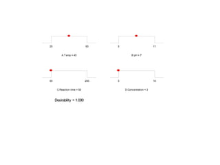
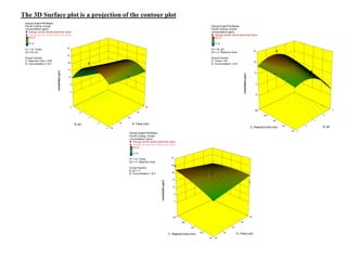
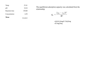
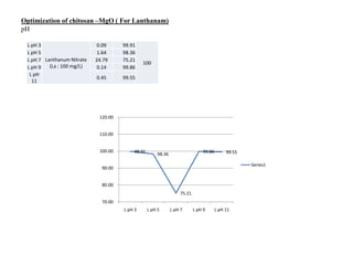
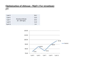


This document describes a study that used response surface methodology (RSM) to optimize the removal of lanthanum metal from wastewater using chitosan-Fe3O4 nanocomposite as an adsorbent. Four variables (adsorbent dose, temperature, pH, and reaction time) were investigated using a Box-Behnken experimental design. Regression analysis identified pH as the most significant factor. Optimization analysis predicted that the maximum lanthanum removal of 91.82% could be achieved at 25.41°C, pH 10.24, 150 minutes reaction time, and 6.5 mg/L lanthanum concentration. A similar RSM study optimized removal of strontium using chitos


