Download to read offline


![Free boson 𝑋(𝑧, 𝑧)
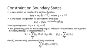
The free boson action is
𝑆 =
1
4𝜋
∫ 𝑑𝑧𝑑𝑧 𝜕𝑋. 𝜕𝑋
Equation of motion is
𝜕𝜕𝑋 = 0 ⇒ 𝜕𝑗 𝑧 = 𝜕𝑗 𝑧 = 0
𝑗 𝑧 = 𝑖𝜕𝑋(𝑧, 𝑧)
𝑗 𝑧 = 𝑖𝜕𝑋(𝑧, 𝑧)
ℎ 𝑋 = 0 and ℎ 𝑗 = ℎ 𝑗 = 1 (𝑗 and 𝑗 are primary fields)
𝑗 𝑧 =
𝑛
𝑧−𝑛−1𝑗𝑛 𝑗 𝑧 =
𝑚
𝑧−𝑚−1𝑗𝑚
𝐿𝑛 and 𝑗𝑚’s are connected as
𝐿𝑛 =
𝑘≻−1
𝑗𝑛−𝑘𝑗𝑘 +
𝑘≤−1
𝑗𝑘𝑗𝑛−𝑘
𝑐 = 1 (by calculating [𝐿𝑛, 𝑗𝑚] and ⟨0|𝐿2𝐿−2|0⟩)
𝑋(𝑧, 𝑧) is expanded as
𝑋 𝑧, 𝑧 = 𝑥0 − 𝑖 𝑗0 ln 𝑧𝑧 + 𝑖
𝑛≠0
1
𝑛
𝑗𝑛𝑧−𝑛
+ 𝑗𝑛𝑧−𝑛
(𝑗0 = 𝑗0)](https://image.slidesharecdn.com/cftpresentation-220406030415/85/Conformal-Boundary-conditions-12-320.jpg)

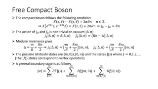
![Free boson on the strip
For variation of action to vary, we have;
∫ 𝑑𝜏 𝜕𝜎𝑋 𝛿𝑋
𝜎=0
𝜎=𝜋
= 0 ⇒
𝜕𝜎𝑋
𝜎=0,𝜋
= 0 (Neumann)
𝛿𝑋
𝜎=0,𝜋
= 𝜕𝜏𝑋
𝜎=0,𝜋
= 0 (Dirichlet)
𝑗𝑛 − 𝑗𝑛 = 0 Neumann − Neumann 𝑗𝑛 + 𝑗𝑛 = 0 Dirichlet − Dirichlet [𝑛 ∈ ℤ]
𝑗𝑛 − 𝑗𝑛 = 0 Neumann − Dirichlet 𝑗𝑛 + 𝑗𝑛 = 0 Dirichlet − Neumann 𝑛 ∈ ℤ +
1
2
We have 𝐿𝑛 = 𝐿𝑛 which implies 𝑇 𝑧 = 𝑇(𝑧).](https://image.slidesharecdn.com/cftpresentation-220406030415/85/Conformal-Boundary-conditions-14-320.jpg)


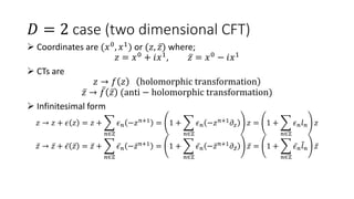
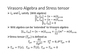
The document discusses conformal field theory (CFT) and its applications, notably in quantum field theory and condensed matter physics. It covers the properties of primary fields, boundary states, and operator product expansions, while also introducing concepts like Virasoro algebra and free bosons. Additionally, it examines boundary conditions and duality in string theory, raising questions about boundary states and their interpretations.


