NumPy arrays can be broadcast together to perform arithmetic operations even if they have different shapes. Broadcasting duplicates smaller arrays to match the shape of larger arrays. It allows arrays with incompatible shapes to still be used together in arithmetic operations. This technique greatly simplifies code. Boolean arrays can be used to select, count, or modify values in NumPy arrays based on logical criteria using techniques like masking and fancy indexing.

1. NumPy Arrays: Broadcasting

2. Introducing Broadcasting
 Arrays with different sizes cannot be added, subtracted, or
generally be used in arithmetic.
 A way to overcome this is to duplicate the smaller array so
that it is the dimensionality and size as the larger array.
 This is called array broadcasting and is available in
NumPy when performing array arithmetic, which can
greatly reduce and simplify your code.

3. Add a scalar to an array
In[2]: a=np.arange(3)
a
Out[2]: array([0, 1, 2])
In[3]: a + 5
Out[3]: array([5, 6, 7])

4. Add a one-dimensional array to a two-
dimensional array
In[4]: M = np.ones((3, 3))
M
Out[4]: array([[ 1., 1., 1.],
[ 1., 1., 1.],
[ 1., 1., 1.]])
In[5]: M + a
Out[5]: array([[ 1., 2., 3.],
[ 1., 2., 3.],
[ 1., 2., 3.]])

5. Visualization of NumPy broadcasting

6. Rules of Broadcasting
 Rule 1: If the two arrays differ in their number of
dimensions, the shape of the one with fewer dimensions is
padded with ones on its leading (left) side.
 Rule 2: If the shape of the two arrays does not match in
any dimension, the array with shape equal to 1 in that
dimension is stretched to match the other shape.
 Rule 3: If in any dimension the sizes disagree and neither
is equal to 1, an error is raised

7. Broadcasting example 1
In[8]: M = np.ones((2, 3))
a = np.arange(3)
The shapes of the arrays are:
M.shape = (2, 3)
a.shape = (3,)
By rule 1 the array a has fewer dimensions, so we pad it on the left with ones:
M.shape -> (2, 3)
a.shape -> (1, 3)
By rule 2, the first dimension disagrees, so we stretch this dimension to match:
M.shape -> (2, 3)
a.shape -> (2, 3)
The shapes match, the final shape will be (2, 3):
In[9]: M + a
Out[9]: array([[ 1., 2., 3.],
[ 1., 2., 3.]])

8. Broadcasting example 2
In[10]: a = np.arange(3).reshape((3, 1))
b = np.arange(3)
the shape of the arrays:
a.shape = (3, 1)
b.shape = (3,)
Rule 1 :pad the shape of b with ones:
a.shape -> (3, 1)
b.shape -> (1, 3)
And rule 2 :upgrade each of these ones to match the corresponding size of
the other array:
a.shape -> (3, 3)
b.shape -> (3, 3)
These shapes are compatible.:
In[11]: a + b
Out[11]: array([[0, 1, 2],
[1, 2, 3],
[2, 3, 4]])

9. Broadcasting example 3
Arrays are not compatible:
In[12]: M = np.ones((3, 2))
a = np.arange(3)
The shapes of the arrays are:
M.shape = (3, 2)
a.shape = (3,)
Again, rule 1 : pad the shape of a with ones:
M.shape -> (3, 2)
a.shape -> (1, 3)
By rule 2, the first dimension of a is stretched to match that of M:
M.shape -> (3, 2)
a.shape -> (3, 3)
Rule 3—the final shapes do not match, so these two arrays are incompatible,:
In[13]: M + a
ValueError

10. NumPy Arrays: Comparisons,
Masks, and Boolean Logic

11.  Masking comes up when you want to extract, modify,
count, or otherwise manipulate values in an array based
on some criterion:
 for example, you might wish to count all values greater
than a certain value, or perhaps remove all out‐ liers that
are above some threshold.
 In NumPy, Boolean masking is often the most efficient way
to accomplish these types of tasks.

12. Comparison Operators as ufuncs
 In[4]: x = np.array([1, 2, 3, 4, 5])
 In[5]: x < 3 # less than
 Out[5]: array([ True, True, False, False, False], dtype=bool)
 In[6]: x > 3 # greater than
 Out[6]: array([False, False, False, True, True], dtype=bool)
 In[7]: x <= 3 # less than or equal
 Out[7]: array([ True, True, True, False, False], dtype=bool)
 In[8]: x >= 3 # greater than or equal
 Out[8]: array([False, False, True, True, True], dtype=bool)
 In[9]: x != 3 # not equal
 Out[9]: array([ True, True, False, True, True], dtype=bool)
 In[10]: x == 3 # equal
 Out[10]: array([False, False, True, False, False], dtype=bool)

13. Comparison Operators as ufuncs

14. Comparison Operators as ufuncs
In[12]: rng = np.random.RandomState(0)
x = rng.randint(10, size=(3, 4))
x
Out[12]: array([[5, 0, 3, 3], [7, 9, 3, 5], [2, 4, 7, 6]])
In[13]: x < 6
Out[13]: array([[ True, True, True, True],
[False, False, True, True],
[ True, True, False, False]], dtype=bool)

15. Working with Boolean Arrays
In[14]: print(x)
[[5 0 3 3]
[7 9 3 5]
[2 4 7 6]]
Counting entries
In[15]: # how many values less than 6?
np.count_nonzero(x < 6)
Out[15]: 8
:In[16]: np.sum(x < 6)
Out[16]: 8
In[17]: # how many values less than 6 in each row?
np.sum(x < 6, axis=1)
Out[17]: array([4, 2, 2])
This counts the number of values less than 6 in each row of the matrix

16. Working with Boolean Arrays
In[18]: # are there any values greater than 8?
np.any(x > 8)
Out[18]: True
In[19]: # are there any values less than zero?
np.any(x < 0)
Out[19]: False
In[20]: # are all values less than 10?
np.all(x < 10)
Out[20]: True
In[21]: # are all values equal to 6?
np.all(x == 6)
Out[21]: False
In[22]: # are all values in each row less than 8?
np.all(x < 8, axis=1)
Out[22]: array([ True, False, True], dtype=bool)

17. Example: Counting Rainy Days
In[1]: import numpy as np
import pandas as pd
# use Pandas to extract rainfall inches as a NumPy array
rainfall = pd.read_csv('data/Seattle2014.csv')['PRCP'].values
inches = rainfall / 254 # 1/10mm -> inches # 1 inch = 25.4
mm
inches.shape
Out[1]: (365,)
In[2]: %matplotlib inline
import matplotlib.pyplot as plt
import seaborn; seaborn.set() # set plot styles
In[3]: plt.hist(inches, 40);

18. Histogram of 2014 rainfall in Seattle

19. Working with Boolean Arrays
Find all days with rain less than 0.5 inches and greater than one inch
In[23]: np.sum((inches > 0.5) & (inches < 1))
Out[23]: 29
In[24]: np.sum(~( (inches <= 0.5) | (inches >= 1) ))
Out[24]: 29
In[25]: print("Number days without rain: ", np.sum(inches == 0))
print("Number days with rain: ", np.sum(inches != 0))
print("Days with more than 0.5 inches:", np.sum(inches > 0.5))
print("Rainy days with < 0.1 inches :", np.sum((inches > 0) & (inches <
0.2)))
Number days without rain: 215
Number days with rain: 150
Days with more than 0.5 inches: 37
Rainy days with < 0.1 inches : 75

20. Boolean Arrays as Masks
In[26]: x
Out[26]: array([[5, 0, 3, 3],
[7, 9, 3, 5],
[2, 4, 7, 6]])
We can obtain a Boolean array for this condition :
In[27]: x < 5
Out[27]: array([[False, True, True, True],
[False, False, True, False],
[ True, True, False, False]], dtype=bool)
masking operation:
In[28]: x[x < 5]
Out[28]: array([0, 3, 3, 3, 2, 4])

21. Boolean Arrays as Masks
In[29]:
# construct a mask of all rainy days
rainy = (inches > 0)
# construct a mask of all summer days (June 21st is the 172nd day)
days = np.arange(365) summer = (days > 172) & (days < 262)
print("Median precip on rainy days in 2014 (inches): ", np.median(inches[rainy]))
print("Median precip on summer days in 2014 (inches): ",
np.median(inches[summer]))
print("Maximum precip on summer days in 2014 (inches): ",
np.max(inches[summer]))
print("Median precip on non-summer rainy days (inches):",
np.median(inches[rainy & ~summer]))
Median precip on rainy days in 2014 (inches): 0.194881889764
Median precip on summer days in 2014 (inches): 0.0
Maximum precip on summer days in 2014 (inches): 0.850393700787
Median precip on non-summer rainy days (inches): 0.200787401575

22. NumPy Arrays: Fancy Indexing

23. Exploring Fancy Indexing
In[1]: import numpy as np
rand = np.random.RandomState(42)
x = rand.randint(100, size=10)
print(x)
[51 92 14 71 60 20 82 86 74 74]
To access three different elements:
In[2]: [x[3], x[7], x[2]]
Out[2]: [71, 86, 14]
Alternatively, we can pass a single list or array of indices
to obtain the same result:
In[3]: ind = [3, 7, 4]
x[ind]
Out[3]: array([71, 86, 60])

24. Exploring Fancy Indexing
Fancy indexing also works in multiple dimensions.
In[5]: X = np.arange(12).reshape((3, 4))
X
Out[5]: array([[ 0, 1, 2, 3],
[ 4, 5, 6, 7],
[ 8, 9, 10, 11]])
Like with standard indexing, the first index refers to the row, and
the second to the column:
In[6]: row = np.array([0, 1, 2])
col = np.array([2, 1, 3])
X[row, col]
Out[6]: array([ 2, 5, 11])

25. Combined Indexing
In[9]: print(X)
[[ 0 1 2 3]
[ 4 5 6 7]
[ 8 9 10 11]]
We can combine fancy and simple indices:
In[10]: X[2, [2, 0, 1]]
Out[10]: array([10, 8, 9])
We can also combine fancy indexing with slicing:
In[11]: X[1:, [2, 0, 1]]
Out[11]: array([[ 6, 4, 5],
[10, 8, 9]])
combine fancy indexing with masking:
In[12]: mask = np.array([1, 0, 1, 0], dtype=bool)
X[row[:, np.newaxis], mask]
Out[12]: array([[ 0, 2],
[ 4, 6],
[ 8, 10]])
X[1:,]
array([[ 4, 5, 6, 7],
[ 8, 9, 10, 11]])

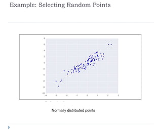
26. Example: Selecting Random Points
In[13]: mean = [0, 0]
cov = [[1, 2],
[2, 5]]
X = rand.multivariate_normal(mean, cov, 100)
X.shape
Out[13]: (100, 2)
In[14]: %matplotlib inline
import matplotlib.pyplot as plt
import seaborn; seaborn.set() # for plot styling
plt.scatter(X[:, 0], X[:, 1]);

27. Example: Selecting Random Points
Normally distributed points

28. Example: Selecting Random Points
In[15]: indices = np.random.choice(X.shape[0], 20,
replace=False) indices
Out[15]: array([93, 45, 73, 81, 50, 10, 98, 94, 4, 64, 65, 89,
47, 84, 82, 80, 25, 90, 63, 20])
In[16]: selection = X[indices] # fancy indexing here
selection.shape
Out[16]: (20, 2)
In[17]: plt.scatter(X[:, 0], X[:, 1], alpha=0.3)
plt.scatter(selection[:, 0], selection[:, 1],
facecolor='none', s=200);

29. Example: Selecting Random Points
Random selection among points