Download to read offline


![Clever indexing
Conceptually, we have a matrix A[i][j] of
tabulated values
This requires two calculations to find indices –
one for i and one for j – and two operations
to lookup values
Combine into a single index
n = 992-32k + j
that can be extracted directly by one bit
manipulation: bits 2 through 14 minus 3040](https://image.slidesharecdn.com/fastphiinverse-100510105727-phpapp02/85/Fast-coputation-of-Phi-x-inverse-10-320.jpg)
![Polynomial evaluation
Taylor approximation:
t = h B(k,j)
x = A(k,j) -0.5 t + 0.125 A(k,j)t2
Rescale B’s by square root of 8:
t = h B’
x = A – c t – A t2 [ c = sqrt(2) ]
Horner’s method:
x = A – t(c – A t)](https://image.slidesharecdn.com/fastphiinverse-100510105727-phpapp02/85/Fast-coputation-of-Phi-x-inverse-11-320.jpg)
![C++ Implementation
double NormalCCDFInverse(double x)
{
float f1 = (float) x;
unsigned int ui;
memcpy(&ui, &f1, 4);
int n = (ui >> 18) - 3008;
ui &= 0xFFFC0000;
float f2;
memcpy(&f2, &ui, 4);
double v = (f1-f2)*B[n];
return A[n] - v*(sqrt2 - A[n]*v);
}](https://image.slidesharecdn.com/fastphiinverse-100510105727-phpapp02/85/Fast-coputation-of-Phi-x-inverse-12-320.jpg)


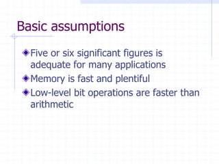
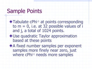
This document summarizes an algorithm for the fast inversion of the normal cumulative distribution function (CDF) based on Marsaglia's method. It represents numbers in a way that allows sample points of the inverse CDF to be extracted via bit manipulation for very fast evaluation. The algorithm tabulates sample values and uses quadratic interpolation between them, indexing the values in a way that can be computed with one bit operation. This allows for inverse CDF computation in less than 5 CPU instructions on most machines.