Downloaded 17 times
![14
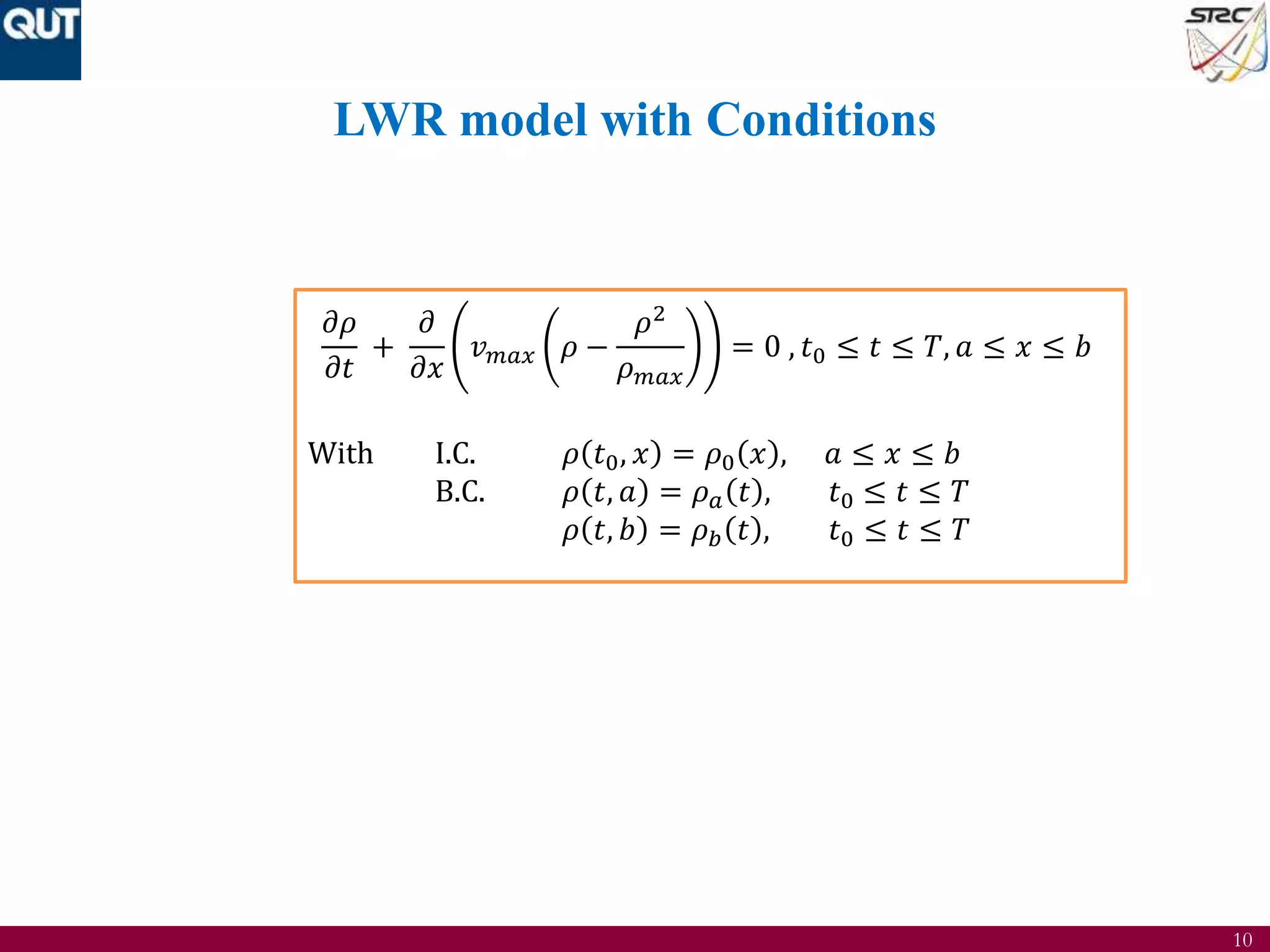
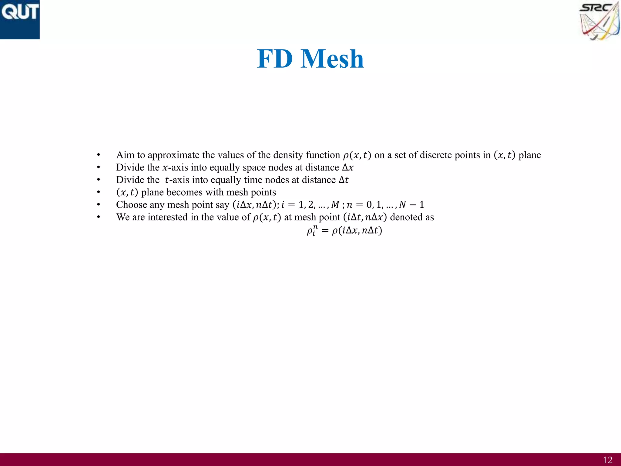
FD Approximations
𝜕𝜌
𝜕𝑡
≈
𝜌𝑖
𝑛+1
−𝜌𝑖
𝑛
∆𝑡
[Forward difference]
𝜕𝜌
𝜕𝑥
≈
𝜌𝑖+1
𝑛
−𝜌𝑖−1
𝑛
2∆𝑥
[Central difference]](https://image.slidesharecdn.com/strcmeeting04-170804021317/75/Mathematical-Understanding-in-Traffic-Flow-Modelling-14-2048.jpg)
![15
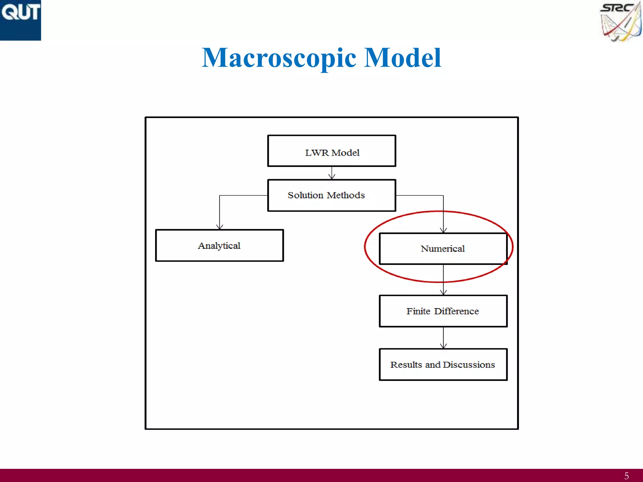
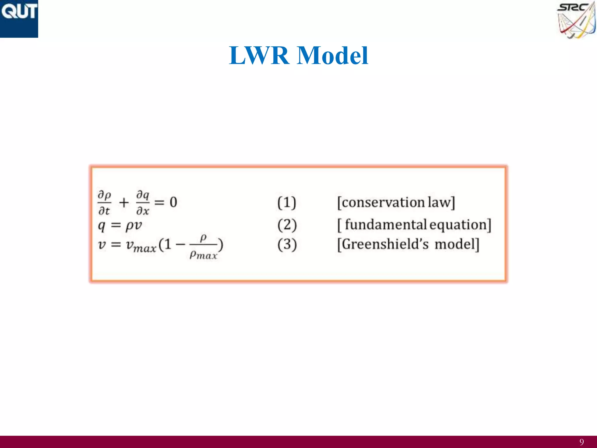
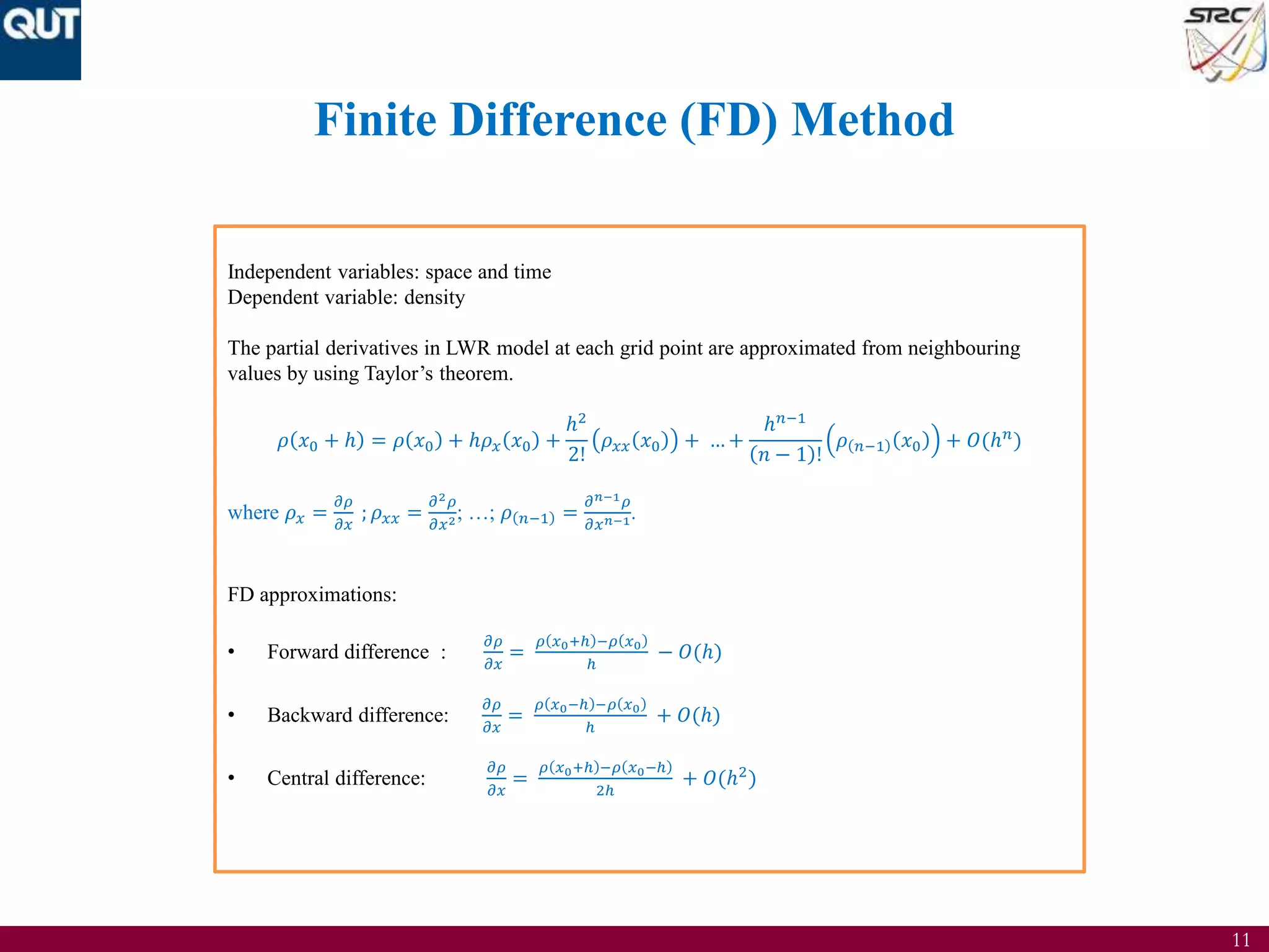
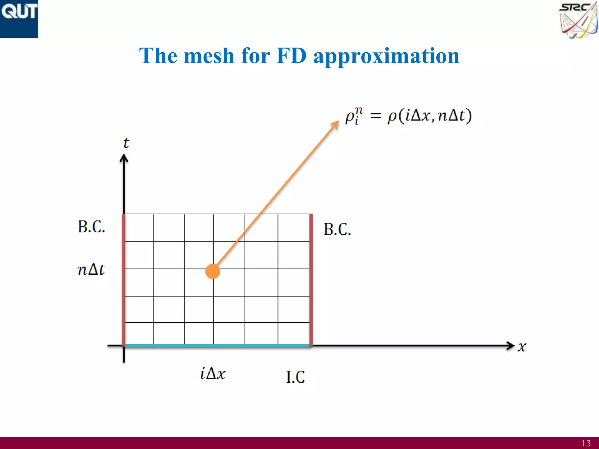
Numerical Solution of LWR Model
𝜌𝑖
𝑛+1
= 𝜌𝑖
𝑛
−
∆𝑡
2∆𝑥
[𝑣 𝑚𝑎𝑥(𝜌𝑖+1
𝑛
−
(𝜌𝑖+1
𝑛
)2
𝜌 𝑚𝑎𝑥
) − 𝑣 𝑚𝑎𝑥(𝜌𝑖−1
𝑛
−
(𝜌𝑖−1
𝑛
)2
𝜌 𝑚𝑎𝑥
)]](https://image.slidesharecdn.com/strcmeeting04-170804021317/75/Mathematical-Understanding-in-Traffic-Flow-Modelling-15-2048.jpg)


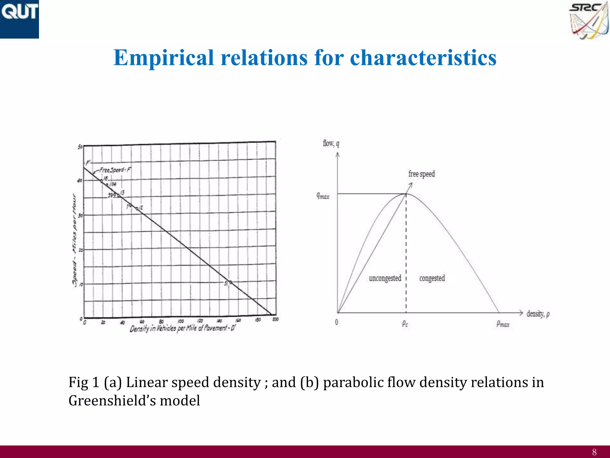
The document discusses the development of mathematical understanding in traffic flow modeling, focusing on both macroscopic and microscopic models. It details various traffic characteristics, fundamental equations, and empirical relations, while also presenting numerical methods such as finite difference for solving the LWR model. Results include traffic density approximations and simulations, demonstrating the model's application in traffic flow analysis.