Downloaded 17 times
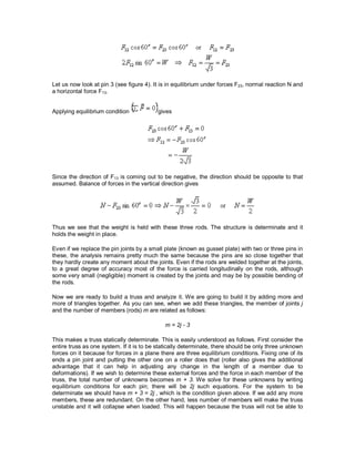

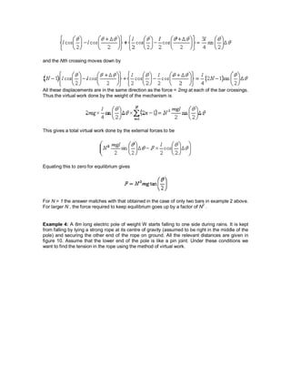
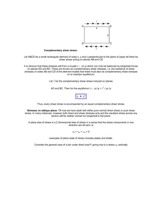
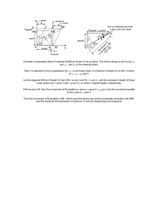
![ = 2xysincos
= xy.2.sincos
(1)
Now resolving forces parallel to PC or in the direction .then xyPC . 1 =xy . PBsin xy . BCcos
ve sign has been put because this component is in the same direction as that of .
again converting the various quantities in terms of PC we have
xyPC . 1 =xy . PB.sin
2
xy . PCcos
2
= [xy (cos
2
sin
2
) ]
= xycos2or (2)
the negative sign means that the sense of is opposite to that of assumed one. Let us examine the
equations (1) and (2) respectively
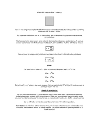
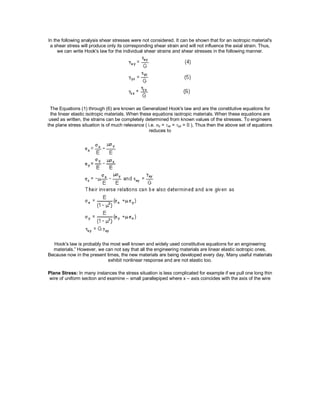
From equation (1) i.e,
= xy sin2
The equation (1) represents that the maximum value of isxy when = 45
0
.
Let us take into consideration the equation (2) which states that
=xy cos2
It indicates that the maximum value of isxy when = 0
0
or 90
0
. it has a value zero when = 45
0
.
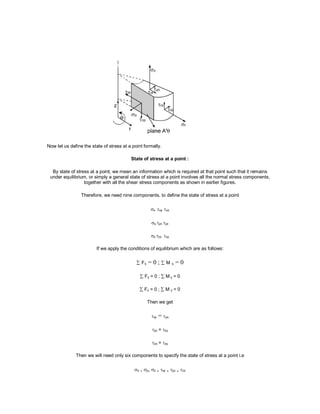
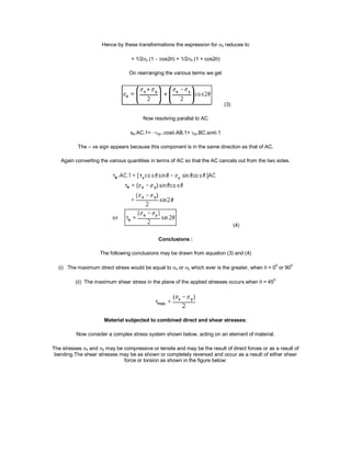
From equation (1) it may be noticed that the normal component has maximum and minimum values of
+xy (tension) and xy (compression) on plane at ± 45
0
to the applied shear and on these planes the
tangential component is zero.
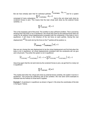
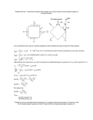
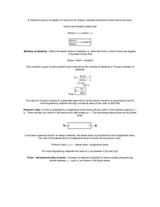
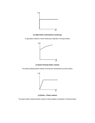
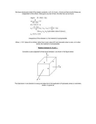
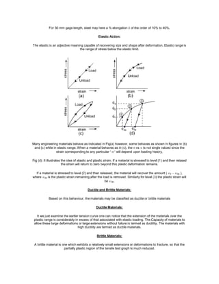
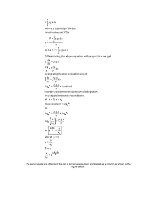
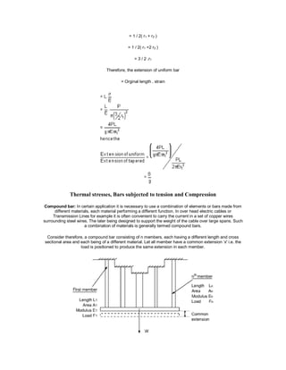
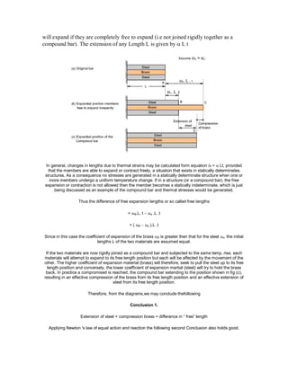
Hence the system of pure shear stresses produces and equivalent direct stress system, one set
compressive and one tensile each located at 450
to the original shear directions as depicted in the figure
below:](https://image.slidesharecdn.com/mos2ndmod-151212070152/85/module-2-Mechanics-39-320.jpg)
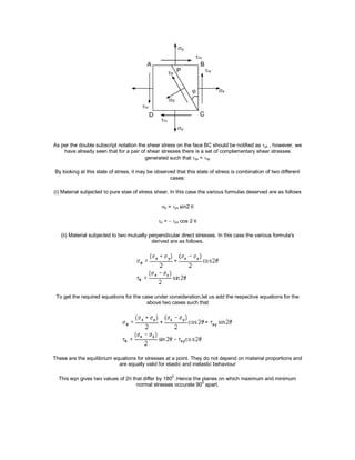
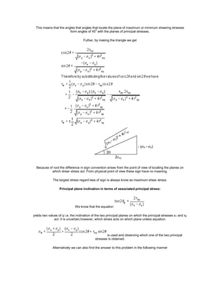
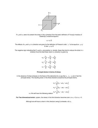
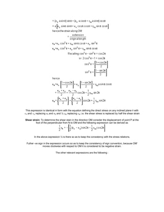
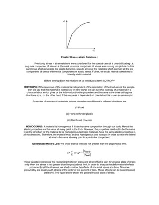
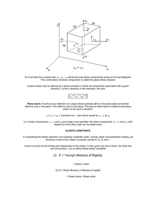
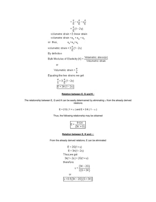
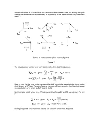
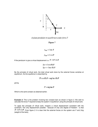
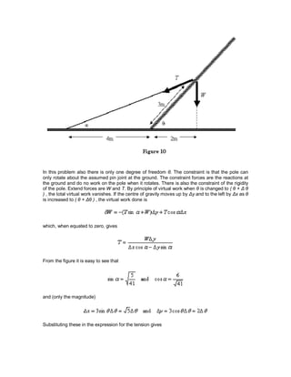
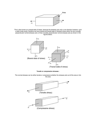
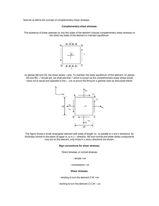
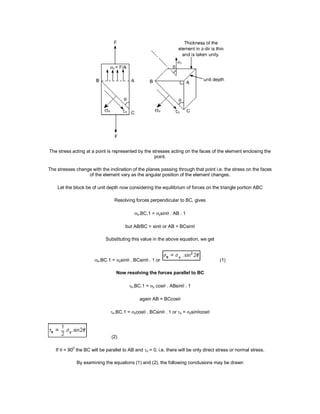
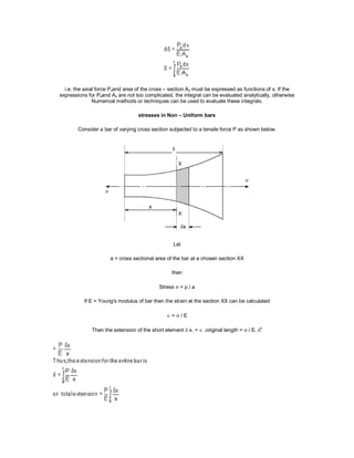
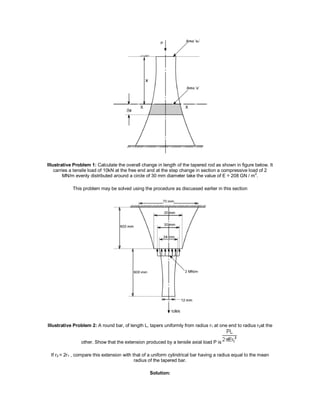
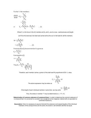
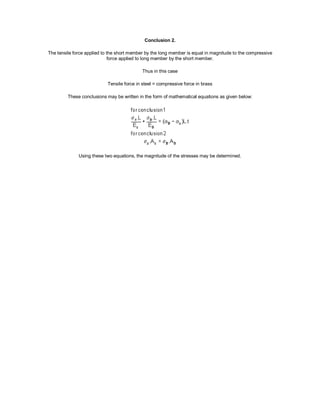
![In this method a line is drawn parallel to the straight line portion of initial stress diagram by off setting this by
an amount equal to 0.2% of the strain as shown as below and this happens especially for the low carbon
steel.
(E) A further increase in the load will cause marked deformation in the whole volume of the metal. The
maximum load which the specimen can with stand without failure is called the load at the ultimate strength.
The highest point ‘E' of the diagram corresponds to the ultimate strength of a material.
u = Stress which the specimen can with stand without failure & is known as Ultimate Strength or Tensile
Strength.
u is equal to load at E divided by the original cross-sectional area of the bar.
(F) Beyond point E, the bar begins to forms neck. The load falling from the maximum until fracture occurs at
F.
[ Beyond point E, the cross-sectional area of the specimen begins to reduce rapidly over a relatively small
length of bar and the bar is said to form a neck. This necking takes place whilst the load reduces, and
fracture of the bar finally occurs at point F ]
Note: Owing to large reduction in area produced by the necking process the actual stress at fracture is often
greater than the above value. Since the designers are interested in maximum loads which can be carried by
the complete cross section, hence the stress at fracture is seldom of any practical value.
Percentage Elongation: ' ':
The ductility of a material in tension can be characterized by its elongation and by the reduction in area at
the cross section where fracture occurs.
It is the ratio of the extension in length of the specimen after fracture to its initial gauge length, expressed in
percent.
lI = gauge length of specimen after fracture(or the distance between the gage marks at fracture)
lg= gauge length before fracture(i.e. initial gauge length)](https://image.slidesharecdn.com/mos2ndmod-151212070152/85/module-2-Mechanics-69-320.jpg)
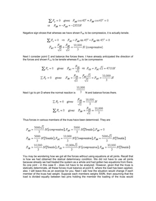
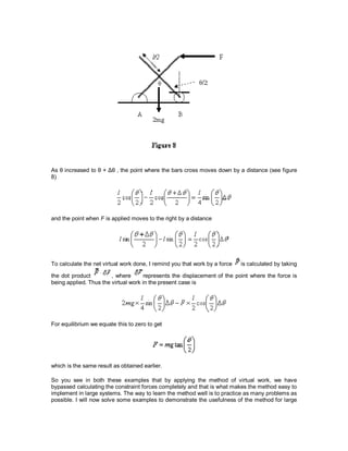
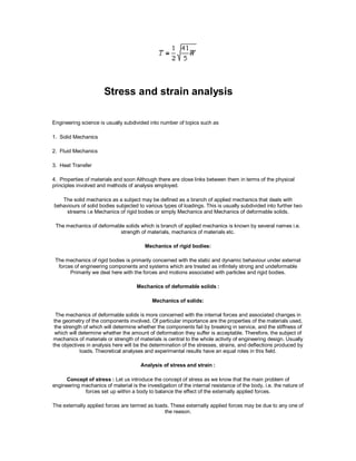
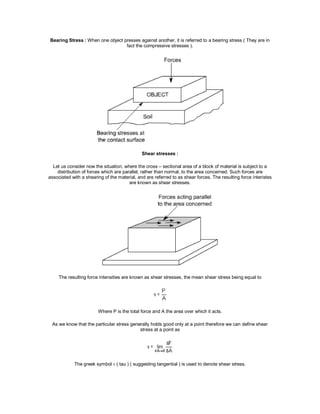
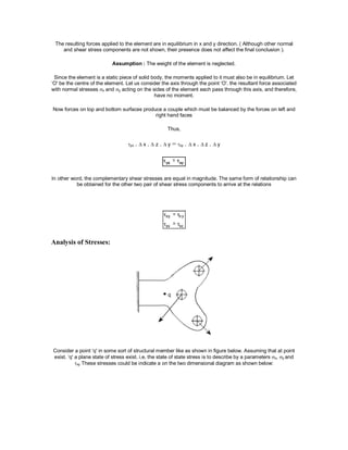
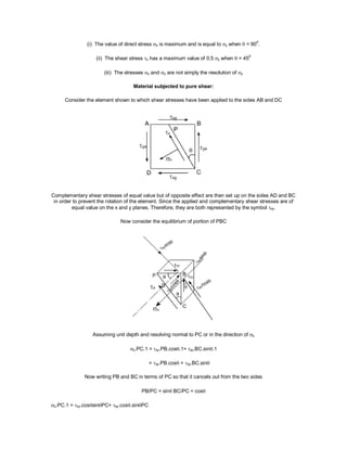
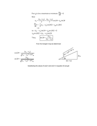
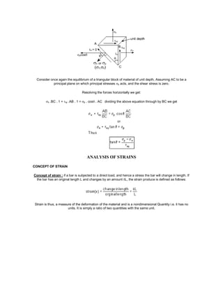
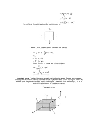
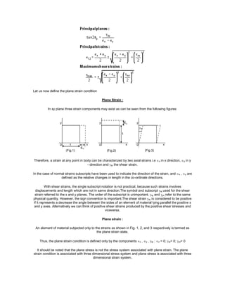
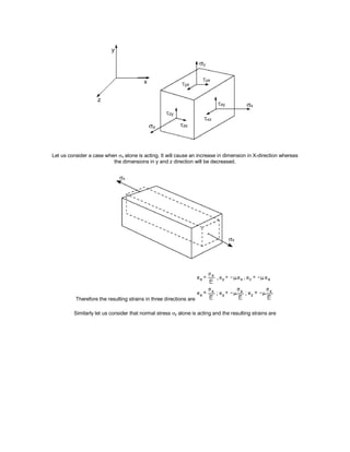
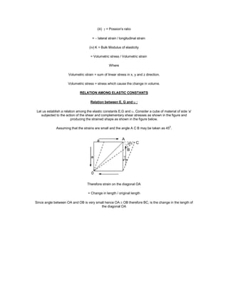
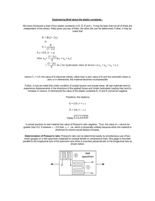
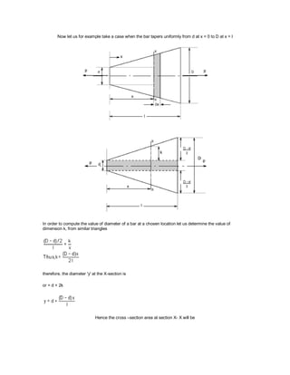
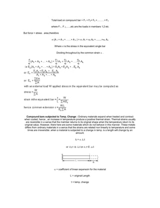
![This type of graph is shown by the cast iron or steels with high carbon contents or concrete.
Members Subjected to Uniaxial Stress
Members in Uni – axial state of stress
Introduction: [For members subjected to uniaxial state of stress]
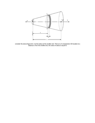
For a prismatic bar loaded in tension by an axial force P, the elongation of the bar can be determined as
Suppose the bar is loaded at one or more intermediate positions, then equation (1) can be readily adapted
to handle this situation, i.e. we can determine the axial force in each part of the bar i.e. parts AB, BC, CD,
and calculate the elongation or shortening of each part separately, finally, these changes in lengths can be
added algebraically to obtain the total charge in length of the entire bar.
When either the axial force or the cross – sectional area varies continuosly along the axis of the bar, then
equation (1) is no longer suitable. Instead, the elongation can be found by considering a deferential element
of a bar and then the equation (1) becomes](https://image.slidesharecdn.com/mos2ndmod-151212070152/85/module-2-Mechanics-71-320.jpg)

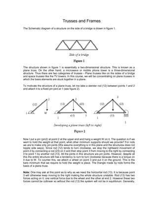
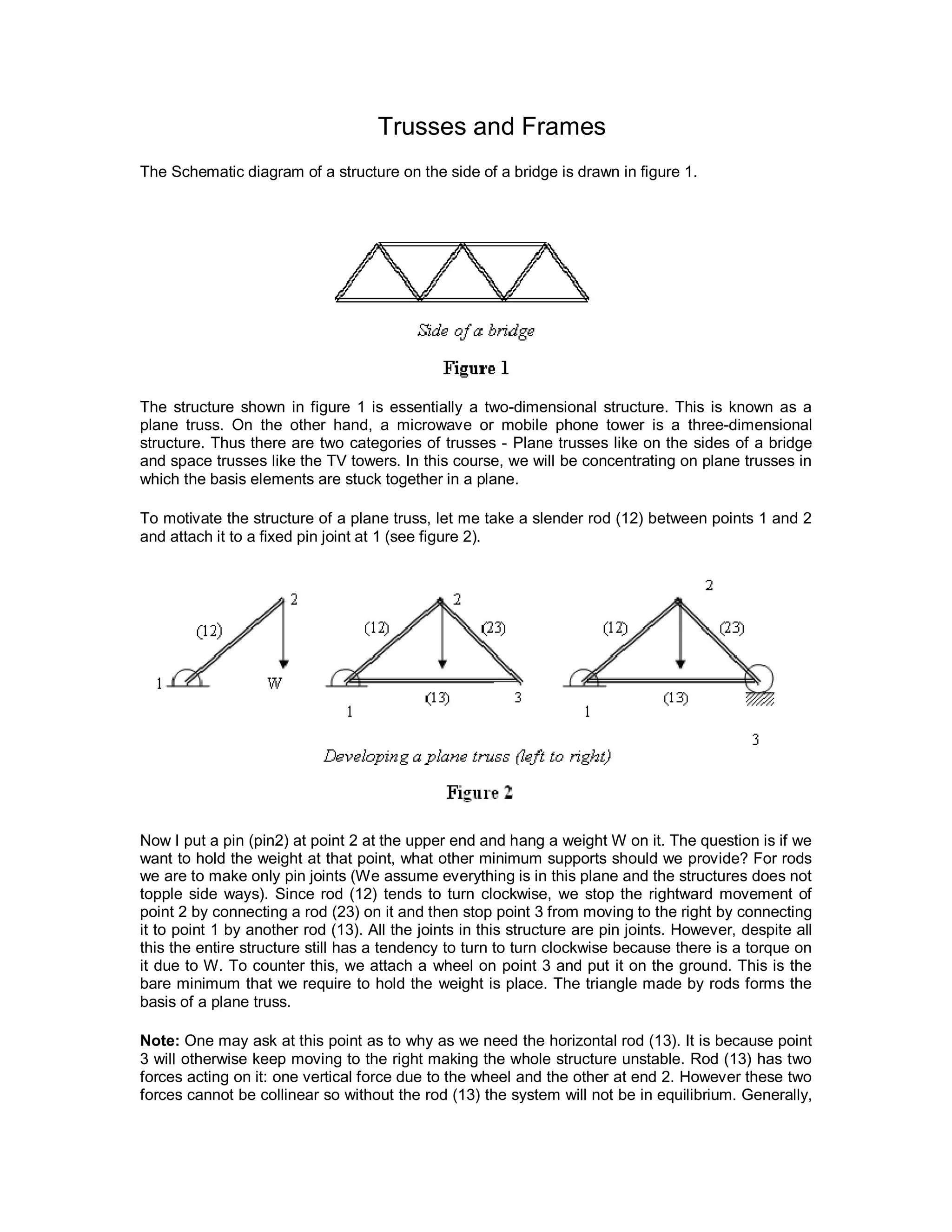
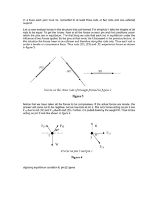
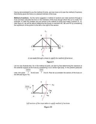
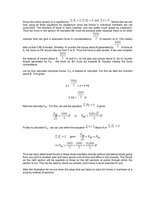
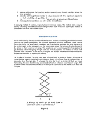
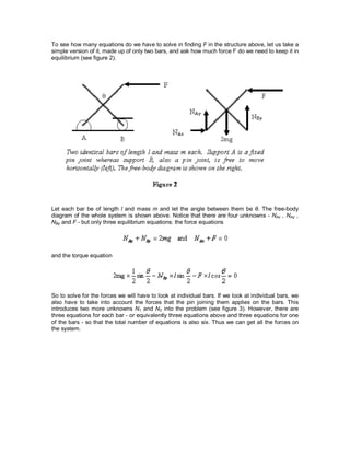
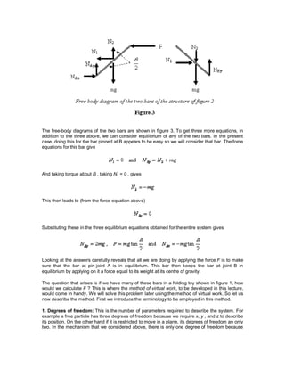
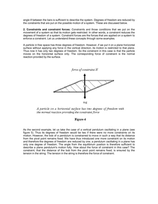
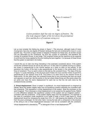
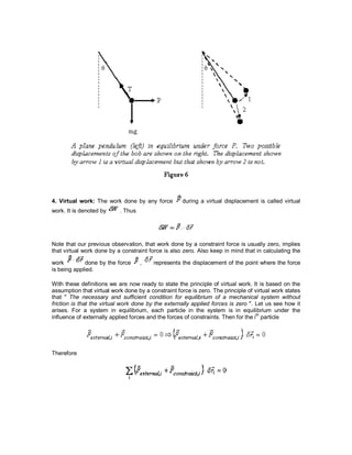
This document discusses trusses and frames. It begins by defining plane trusses, which are two-dimensional structures like the sides of a bridge, and space trusses, which are three-dimensional structures like TV towers. It then motivates the structure of a plane truss using a simple example of three rods connected in a triangle. The document goes on to analyze the forces in this simple truss and introduces the method of joints and method of sections for analyzing more complex trusses. It concludes by introducing the method of virtual work, which provides an alternative way to determine forces without considering the equilibrium of individual parts of the structure.
![THEORY OF STRUCTURES-I [B. ARCH.]](https://cdn.slidesharecdn.com/ss_thumbnails/theoryofstructures-ib-180903021950-thumbnail.jpg?width=640&height=640&fit=bounds)