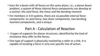
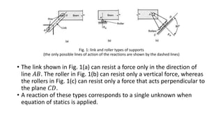
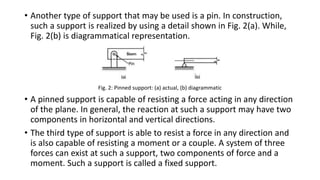
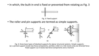
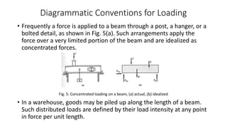
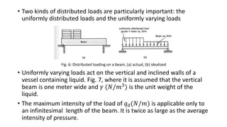
1. A beam can experience three internal forces at a section - axial force, shear, and bending moment. Even for planar beams, all three forces may develop. 2. There are three types of supports - roller/link, pin, and fixed. Roller/link supports resist one force, pin supports resist two forces, and fixed supports resist two forces and a moment. 3. Beams can experience different load types - concentrated, uniform distributed, and varying distributed loads. Methods are presented to calculate the shear, axial, and bending effects of these loads on beams.

1. Chapter 5
Axial Force, Shear, and Bending Moment
Mechanics of Solids

2. • Even for a beam with all forces on the same plane, i.e., a planar beam
problem, a system of three internal force components can develop at
a section: the axial force, the shear and the bending moment
• For members in 3-D systems, there are six possible internal force
components: an axial force, two shear components, two bending
moment components, and a torque.
Part A - Calculation of Reaction
• 3 types of supports for planar structures, identified by the kind of
resistance they offer to the forces.
• One type of support is physically realized by a roller or a link. It is
capable of resisting a force in only one specific line of action.

3. Fig. 1: link and roller types of supports
(the only possible lines of action of the reactions are shown by the dashed lines)
• The link shown in Fig. 1(a) can resist a force only in the direction of
line 𝐴𝐵. The roller in Fig. 1(b) can resist only a vertical force, whereas
the rollers in Fig. 1(c) can resist only a force that acts perpendicular to
the plane 𝐶𝐷.
• A reaction of these types corresponds to a single unknown when
equation of statics is applied.

4. • Another type of support that may be used is a pin. In construction,
such a support is realized by using a detail shown in Fig. 2(a). While,
Fig. 2(b) is diagrammatical representation.
Fig. 2: Pinned support: (a) actual, (b) diagrammatic
• A pinned support is capable of resisting a force acting in any direction
of the plane. In general, the reaction at such a support may have two
components in horizontal and vertical directions.
• The third type of support is able to resist a force in any direction and
is also capable of resisting a moment or a couple. A system of three
forces can exist at such a support, two components of force and a
moment. Such a support is called a fixed support.

5. • In which, the built-in end is fixed or prevented from rotating as Fig. 3
Fig. 3: Fixed support
• The roller and pin supports are termed as simple supports.
Fig. 4: three basic types of idealized supports for planar structural systems. Simple supports:
(a) a pinned support resists two force components, and (b) a roller or a link resists only one directed force
Fixed support: (c) it resists two force components and a moment

6. Diagrammatic Conventions for Loading
• Frequently a force is applied to a beam through a post, a hanger, or a
bolted detail, as shown in Fig. 5(a). Such arrangements apply the
force over a very limited portion of the beam and are idealized as
concentrated forces.
Fig. 5: Concentrated loading on a beam, (a) actual, (b) idealized
• In a warehouse, goods may be piled up along the length of a beam.
Such distributed loads are defined by their load intensity at any point
in force per unit length.

7. • Two kinds of distributed loads are particularly important: the
uniformly distributed loads and the uniformly varying loads
Fig. 6: Distributed loading on a beam, (a) actual, (b) idealized
• Uniformly varying loads act on the vertical and inclined walls of a
vessel containing liquid. Fig. 7, where it is assumed that the vertical
beam is one meter wide and 𝛾 (𝑁/𝑚3
) is the unit weight of the
liquid.
• The maximum intensity of the load of 𝑞0(𝑁/𝑚) is applicable only to
an infinitesimal length of the beam. It is twice as large as the average
intensity of pressure.

8. Fig. 7: Hydrostatic loading on a vertical wall
• The total force exerted by such a loading on a beam is 𝑞0ℎ 2 N, and
its resultant acts at a distance h/3 above the vessel’s bottom.
Horizontal bottoms of vessels containing liquid are loaded uniformly.
various aerodynamic loadings are of distributed types.
• It is conceivable to load a beam with a concentrated moment applied
to the beam essentially at a point. Consider, Fig. 8(a) and its
diagrammatic representation shown in Fig. 8(c).

9. Fig. 8: A method for applying a concentrated moment to a beam
• In Fig. 9, to maintain the applied force 𝑃 in the equilibrium at joint 𝐶,
a shear 𝑃 and a moment 𝑃𝑑 must be developed at the support, Fig.
9(c). These forces apply a concentrated moment and an axial force, as
shown in Fig. 9(b)

10. Classification of Beams
Fig. 9: loaded horizontal member applies an applied force and a concentrated moment to the vertical member
• If the supports at the ends of a beam are either pins or rollers, the
beams are simply supported, or simple beams, Figs. 10(a) and (b)
• Fixed beam, if the ends have fixed supports, Fig. 10(c)

11. Fig. 10: Types of Beams
• Restrained beams, one end is fixed and other is simply supported, Fig.
10(d). This beam is restrained from rotation.
• Cantilever beam, fixed at one end and completely free at the other
end, Fig. 10(e)

12. • If the beam projects beyond a support, Overhanging beam, Fig. 10(f)
• If intermediate supports are provided for a physically continuous
member acting as a beam, Fig. 10(g), Continuous beam.
• The distance 𝐿, between supports is called a span. In a continuous
beam, there are several spans that may be of varying lengths.
• The beam shown in Fig. 10(a) is a simple beam with a concentrated
load, whereas the beam in Fig. 10(b) is a simple beam with a
uniformly distributed load.
• If for a planar beam or a frame, the number of unknown reaction
components, including a bending moment, does not exceed three,
such a system is externally statically determinate.
• These unknowns can be found from the equations of static
equilibrium.

13. Calculation of Beam Reactions
• When all the forces are applied in one plane, three equations of static
equilibrium are available for the analysis.
𝐹𝑥 = 0 , 𝐹𝑦 = 0 , 𝑀𝑧 = 0
• From straight beams in the horizontal position, the x-axis will be taken
in an horizontal direction, the y-axis in the upward vertical direction,
and the z-axis normal to the plane of the paper.
• The deformation of beams, being small, is neglected when the
equations of statics are applied.

14. Part B - Direct Approach for Axial Force, Shear and
Bending Moment
Application of the method of sections
• The analysis of any beam or frame for determining the internal forces
begins with the preparation of a free-body diagram showing both the
applied and the reactive forces.
• If a whole body is in equilibrium, any part of it is likewise in
equilibrium.
• Consider a beam shown in Fig. 11, with certain concentrated and
distributed forces acting on it. The reactions can be computed using
equations of static equilibrium. At a section of such a member, a
vertical force, a horizontal force, and a moment are necessary to
maintain the isolated part in equilibrium.

15. Axial Force in Beams
Fig. 11: An application of the method of sections to a statistically
determinate beam

16. • A horizontal force such as 𝑃, shown in Fig. 11(b) and (c) may be
necessary at section of a beam to satisfy the conditions of
equilibrium. The magnitude and sense of this force follows from a
particular solution of the equation, 𝐹𝑥 = 0.
• If the horizontal force 𝑃 acts towards the section, it is called a ‘thrust’;
if away, it is called ‘axial tension’.
• It is imperative to apply this force through the centroid of the cross-
sectional area of the member to avoid bending.
• The line of action of the axial force will always be directed through
the centroid of the beam’s cross-sectional area.
• The tensile force at a section is customarily taken positive.
• The axial force (thrust) at section 𝑋 − 𝑋 in Figs. 11(b) and (c) is equal
to the horizontal force 𝑃2.

17. Shear in Beams
• To maintain a segment of a beam, as shown in Fig. 11(b), in
equilibrium, there must be an internal vertical force 𝑉, acting at right
angles to the axis of the beam, is called the shear force.
• The shear is numerically equal to the algebraic sum of all the vertical
components of the external forces acting on the isolated segment,
but it is opposite in direction.
• Given the qualitative data shown in Fig. 11(b), 𝑉 is opposite in the
direction to the downward load to the left of the section. This shear
may also be computed by considering the right hand segment shown
in Fig. 11(c).
• The same shear shown in Figs. 11(b) and (c) at the section 𝑋 − 𝑋 is
opposite in direction in the two diagrams.

18. • For the part of the downward load 𝑊1 to the left of section 𝑋 − 𝑋,
the beam at the section provides an upward support to maintain
vertical forces in equilibrium. Conversely, the loaded portion of the
beam exerts a downward force on the beam, as shown in Fig. 11(c)
• A reversal in the direction of shear takes place at one section or
another along a beam.
• A downward internal force 𝑉 acting at a section on an isolated left
section of the beam, as in Fig. 12(a), or an upward force 𝑉 acting at
the same section on the right segment of the beam, as in Fig.
12(b),corresponds to positive shear.
• Positive shears are shown in Fig. 12(c) for an element isolated from a
beam by two sections, and again in Fig. 12(d).
• The shear at section 𝑋 − 𝑋 of Fig. 11(a) is a negative shear. It is
essential to associate the direction with a particular side of a section.

19. Fig. 13: Positive sense of shear and bending
Fig. 12: Definition of positive shear moment defined in (a) is used in this text with
coordinates shown in (b)
• The selected sign convention for shear appears to be based on
directing the coordinate axis as shown in Fig. 13(a).
• A few books reverse the direction of positive shear to be consistent
with the direction of axes in Fig. 13(b)

20. Bending Moment in Beams
• The internal shear and axial forces at a section of a beam satisfy only
two equations of equilibrium: 𝐹𝑥 = 0 and 𝐹𝑦 = 0
• The remaining condition of a static equilibrium for a planar problem is
𝑀𝑧 = 0. This can be satisfied only by developing a couple or an
internal resisting moment within the cross-sectional area of the cut to
counteract the moment caused by the external forces.
• These moments tend to bend a beam in the plane of the loads and
are usually referred as ‘bending moments’.
• To determine an internal bending moment maintaining a beam
segment in equilibrium, either the left- or the right-hand part of a
beam free-body can be used, as shown in Figs. 11(b) and (c).

21. • The magnitude of the bending moment is found by summation of the
moments caused by all forces multiplied by their respective arms.
• The internal forces 𝑉 and 𝑃, as well as the applied couples, must be
included in the sum.
• In order to exclude the moments caused by 𝑉 and 𝑃, it is
advantageous to select the point of intersection of these two internal
forces as the point around which the moments are summed. This
points lies on the centroidal axis of the beam cross-section.
• In Figs. 14(b) and (c), the internal bending moments shown cause
tension in the upper part of the beam and compression in the lower.
• A continuous occurrence of such moments along the beam makes the
beam deform convex upwards, i.e., ‘shed water’. Such bending
moments are assigned a negative sign, Fig. 14(c)

22. Fig. 14: definition of bending moment signs
• A positive moment is defined as one that produces compression in
the top part and tension in the lower part of a beam’s cross-section.
The beam assumes a shape that ‘retains water’, Fig. 14(b)
• As for shears 𝑉, in addition to the sense of 𝑀, it is also essential to
associate the moment for a particular side of a section.

23. Axial-Force, Shear, and Bending-Moment
Diagrams
• Using the obtained magnitude and the sign conventions adopted for
these quantities, a plot of their values may be made on separate
diagrams.
• On such diagrams, ordinates may be laid off equal to the computed
quantities from a base line representing the length of a beam.
• It is convenient to make these plots directly below the free-body
diagram of the beam, using the same horizontal scale for the length
of the beam.
• The procedure of sectioning a beam or a frame and finding the
system of forces at the section is the most fundamental approach.

24. Part C- Shear and Bending Moments by
Integration
Differential Equations of Equilibrium for a Beam Element
• Consider a beam element ∆𝑥 long, isolated by two adjoining sections
taken perpendicular to its axis, Fig. 15(b). Such an element is shown
as a free-body in Fig. 15(c).
• All the forces shown acting on this element have positive sense. As
the shear and the moment may each change from one section to the
next, on the right side of the element, these quantities are,
respectively, 𝑉 + ∆𝑉 and 𝑀 + ∆𝑀.

25. Fig. 15: Beam and beam-elements between adjoining sections
• From the condition for equilibrium of vertical forces,
𝐹𝑦 = 0 ↑ + 𝑉 + 𝑞 ∆𝑥 − 𝑉 + ∆𝑉 = 0
or
∆𝑉
∆𝑥
= 𝑞

26. • For equilibrium, the summation of moments around 𝐴 must be zero.
• From point 𝐴 the arm of the distributed forces is ∆𝑥/2, one has
𝑀𝐴 = 0 ↺ + 𝑀 + ∆𝑀 − 𝑉∆𝑥 − 𝑀 − 𝑞 ∆𝑥 ∆𝑥 2 = 0
or
∆𝑀
∆𝑥
= 𝑉 +
𝑞 ∆𝑥
2
• In above equations, in the limit as ∆𝑥 → 0 yield the following two
basic differential equations:
𝑑𝑉
𝑑𝑥
= 𝑞 and
𝑑𝑀
𝑑𝑥
= 𝑉 ⟹
𝑑2 𝑀
𝑑𝑥2 =
𝑑𝑉
𝑑𝑥
= 𝑞
• These differential equations can be used for determining reactions of
statically determinate beams from boundary conditions.

27. Shear Diagrams by Integration of the Load
𝑉 =
0
𝑥
𝑞 𝑑𝑥 + 𝐶1
• It is seen that the shear at a section is simply an integral (i.e., a sum)
of the vertical forces along the beam from the left end of the beam to
the section plus a constant of integration 𝐶1. This constant is equal to
the shear on the left-hand end.
• If no force occurs between any two sections, no change in the
amount of shear takes place. If a concentrated force comes into the
summation, a discontinuity, or a ‘jump’ in the value of shear occurs.
• The shear at a section is simply equal to the sum of all vertical forces
to the left of the section.

28. Fig. 16: Shear diagrams for (a) a uniformly distributed load intensity, and
(b) a uniformly increasing load intensity
• If the applied load acts upward, the slope of the shear diagram is
positive, and vice versa. The slope is equal to the corresponding
applied load intensity.

29. • Consider a segment of a beam with a uniformly distributed
downward load 𝑤0 and known shears at both ends, as shown in Fig.
16(a). Since here the applied load intensity 𝑤0 is negative and
uniformly distributed, i.e., 𝑞 = −𝑤0 = 𝑐𝑜𝑛𝑠𝑡𝑎𝑛𝑡, the slope of the
shear diagram exhibits the same characteristics.
• The linearly varying load intensity acting upward on a beam segment
with known shears at the ends has a diagram as shown in Fig. 16
• The locally applied upward load 𝑞1 is smaller than the corresponding
one 𝑞2 near the right end. Therefore, the positive slope of the shear
diagram on the left is smaller than it is on the right, and the shear
diagram is concave upward.
• When the consecutive summation process is used, the diagram must
end up with the previously calculated shear (reaction) at the right end
of a beam.

30. Moment Diagrams by Integration of the Shear
𝑀 =
0
𝑥
𝑉 𝑑𝑥 + 𝐶2
• Where 𝐶2 is a constant of integration corresponding to boundary
conditions at 𝑥 = 0.
• The meaning of the term 𝑉 𝑑𝑥 is shown graphically by the hatched
areas of the shear diagrams in Fig. 17. The summation of these areas
between definite sections through a beam corresponds to an
evaluation of the definite integral.
• If the ends of a beam are on rollers, pin-ended, or free, the starting
and the terminal moments are zero.
• If the end is built-in (fixed against rotation), in statically determinate
beams, the end moment is known from the reaction calculations.

31. • If the fixed end of the beam is on the left, this moment with the
proper sign is the initial constant of integration 𝐶2.
Fig. 17: Shear and moment diagrams for (a) a uniformly distributed load intensity, and
(b) a uniformly increasing load intensity

32. • By proceeding continuously along the beam from the left-hand end
and summing up the areas of the shear diagram with due regard to
their sign, the moment is obtained.
• The change in moment in a given segment of a beam is equal to the
area of the corresponding shear diagram.
• The slopes of the diagram have the same sign and magnitude as the
corresponding shears on the shear diagram, since 𝑑𝑀 𝑑𝑥 = 𝑉.
• If no shear occurs along a certain portion of a beam, no change in
moment takes place.
• The maximum or minimum moment occurs where the shear is zero.
• In a bending-moment diagram obtained by summation, at the right-
hand end of the beam, the terminal conditions for the moment must
be satisfied.

33. • If the end is free or pinned, the computed sum must equal to zero.
• If the end is built-in, the end moment computed by summation
equals the one calculated initially for the reaction.
Effect of Concentrated Moments on Moment Diagrams
• If there is external concentrated moment acting on the infinitesimal
element, the derived summation process applies only up to the point
of application of an external moment.
• At a section just beyond an externally applied moment, a different
bending moment is required to maintain the segment of a beam in
equilibrium.

34. Fig. 18: An external concentrated moment acting on an element of a beam
• In above Fig. 18, an external clockwise moment 𝑀𝐴 is acting on the
element of a beam at 𝐴. Then, if the internal clockwise moment in
the left is 𝑀 𝑂, for equilibrium of the element, the resisting counter-
clockwise moment on the right must be 𝑀 𝑂 + 𝑀𝐴.
• At the point of the externally applied moment, a discontinuity, or a
‘jump’, equal to the concentrated moment appears in the moment
diagram.
• After the discontinuity in the moment-diagram is passed, the
summation process of the shear-diagram areas may be continued
over the remainder of the beam.

35. Moment Diagram and the Elastic Curve
• The shape of the deflected axis of a beam can be established from the
sign of the moment diagram.
• The trace of the axis of a loaded elastic beam in a deflected position is
known as the elastic curve.
Fig. 19: (b) Shear and (c) bending-moment diagrams for (a) the symmetrically loaded beam
• An inspection of Fig. 19(c) shows that the bending moment
throughout the length of the beam is positive. Accordingly, the elastic
curve shown in Fig. 19(d) is concave up at every point.

36. Fig. 20: (b) Axial-force, (c) Shear and (d) bending-moment diagrams for (a) the loaded beam

37. • In a more complex diagram, Fig. 20(d), zones of positive and negative
moment occur.
• Corresponding to the zones of negative moment, a definite curvature
of the elastic curve that is concave down takes place, Fig. 20(e).
• on the other hand, for the zone 𝐻𝐽, where the positive moment
occurs, the concavity of the elastic curve is upward.
• Where curves join, as at 𝐻 and 𝐽, there are lines that are tangent to
the two joining curves since the beam is physically continuous.
• The free end 𝐹𝐺 of the beam is tangent to the elastic curve at 𝐹.
There is no curvature in 𝐹𝐺, since the moment is zero in that segment
of the beam.
• The point of transition on the elastic curve into reverse curvature is
called the ‘point of inflection’ or ‘contraflexure’. At this point, the
moment changes its sign, and the beam is not called upon to resist
any moment.

38. Singularity Functions
• If the loading 𝑞 𝑥 is a continuous function between the supports,
solution of the differential equation 𝑑2 𝑀 𝑑𝑥2 = 𝑑𝑉 𝑑𝑥 = 𝑞 𝑥 is a
convenient approach for determining 𝑉 𝑥 and 𝑀 𝑥 .
• If the loading function is discontinuous, the notation of operational
calculus can be used. The function 𝑞 𝑥 considered here are
polynomials with integral powers of 𝑥.
Fig. 21: A loaded beam

39. • Consider a loaded beam as in Fig. 21. Since the applied loads are
point (concentrated) forces, four distinct regions exist to which
different bending moment expressions apply. These are
𝑀 = 𝑅1 𝑥 when 0 ≤ 𝑥 ≤ 𝑑
𝑀 = 𝑅1 𝑥 − 𝑃1 𝑥 − 𝑑 when d ≤ 𝑥 ≤ 𝑏
𝑀 = 𝑅1 𝑥 − 𝑃1 𝑥 − 𝑑 + 𝑀 𝑏 when b ≤ 𝑥 ≤ 𝑐
𝑀 = 𝑅1 𝑥 − 𝑃1 𝑥 − 𝑑 + 𝑀 𝑏 + 𝑃2 𝑥 − 𝑐 when c ≤ 𝑥 ≤ 𝐿
• All four equations can be written as one using the following symbolic
function:
𝑥 − 𝑎 𝑛 =
0
𝑥 − 𝑎 𝑛
for 0 ≤ 𝑥 ≤ 𝑎
for 𝑎 ≤ 𝑥 ≤ ∞
where 𝑛 ≥ 0 𝑛 = 0, 1, 2, . . . .

40. • The expression enclosed by the pointed brackets does not exist until
𝑥 reaches 𝑎. For 𝑥 beyond 𝑎, the expression becomes an ordinary
binomial. For 𝑛 = 0 and for 𝑥 > 𝑎, the function is unity.
• On this basis, the four separate functions for 𝑀 𝑥 given for the beam
of Fig. 21 can be combined into one expression that is applicable
across the whole span:
𝑀 = 𝑅1 𝑥 − 0 1
− 𝑃1 𝑥 − 𝑑 1
+ 𝑀 𝑏 𝑥 − 𝑏 0
+ 𝑃2 𝑥 − 𝑐 1
Here the values of 𝑎 are 0, 𝑑, 𝑏, and 𝑐, respectively.
• To work with this function further, it is convenient to introduce two
additional symbolic functions. One is for the concentrated force,
treating it as a degenerate case of a distributed. The other is for the
concentrated moment, treating it similarly.

41. Fig. 22: Concentrated force 𝑃 and moment 𝑀 𝑎: (a) and (b) considered as distributed load, and
(c) Symbolic notation for 𝑃 and 𝑀 at 𝑎
• A concentrated (point) force may be considered as an enormously
strong distributed load acting over a small interval 𝜀, Fig. 22 (a). By
treating 𝜀 as a constant,
lim
𝜀→0 𝑎− 𝜀 2
𝑎+𝜀/2
𝑃
𝜀
𝑑𝑥 = 𝑃

42. • 𝑃 𝜀 has the dimensions of force per unit distance such as lb/in, and
corresponds to the distributed load 𝑞 𝑥 in the earlier treatment.
• As 𝑥 − 𝑎 1 → 0, by an analogy of 𝑥 − 𝑎 1 to 𝜀, for a concentrated
force at 𝑥 = 𝑎,
𝑞 = 𝑃 𝑥 − 𝑎 ∗
−1
• For 𝑞, this expression is dimensionally correct, although 𝑥 − 𝑎 ∗
−1 at
𝑥 = 𝑎 becomes infinite and by definition is zero everywhere else.
Thus, it is a singular function.
• The asterisk subscript of the bracket is a remainder that, the integral
of this expression extending over the range 𝜀 remains bounded and
upon integration, yields the point force itself.
• Therefore, a special symbolic rule of integration must be adopted:
0
𝑥
𝑃 𝑥 − 𝑎 ∗
−1 = 𝑃 𝑥 − 𝑎 0

43. • The coefficient 𝑃 is known as the strength of singularity.
• For 𝑃 equal to unity, the unit point load function 𝑥 − 𝑎 ∗
−1 is also
called the Dirac delta or unit impulse function.
• By analogous reasoning, Fig. 22(b), the loading function 𝑞 for
concentrated moment at 𝑥 = 𝑎 is
𝑞 = 𝑀 𝑎 𝑥 − 𝑎 ∗
−2
• This function in being integrated twice defines two symbolic rules of
integration.
0
𝑥
𝑀 𝑎 𝑥 − 𝑎 ∗
−2 𝑑𝑥 = 𝑀 𝑎 𝑥 − 𝑎 ∗
−1
0
𝑥
𝑀 𝑎 𝑥 − 𝑎 ∗
−1 𝑑𝑥 = 𝑀 𝑎 𝑥 − 𝑎 ∗
0

44. • The expression of 𝑞 is correct dimensionally since 𝑞 has the units of
lb/in.
• For 𝑀 𝑎 equal to unity, one obtains the unit point moment function,
𝑥 − 𝑎 ∗
−2, which is also called the doublet or dipole. This function is
also singular being infinite at 𝑥 = 𝑎 and zero elsewhere. However
after integrating twice, a bounded result is obtained.
• The integral of binomial functions in pointed brackets for 𝑛 ≥ 0 is
given by:
0
𝑥
𝑥 − 𝑎 𝑛 𝑑𝑥 =
𝑥 − 𝑎 𝑛 + 1
𝑛 + 1
for 𝑛 ≥ 0
• This integration process is shown in Fig. 23. if the distance 𝑎 is set
equal to zero, one obtains conventional integrals.

45. Fig. 23: Typical integrations