Downloaded 324 times
![NATIONAL CHENG KUNG UNIVERSITY
Inst. of Manufacturing Information & Systems
DIGITAL IMAGE PROCESSING AND SOFTWARE
IMPLEMENTATION
HOMEWORK 1
Professor name: Chen, Shang-Liang
Student name: Nguyen Van Thanh
Student ID: P96007019
Class: P9-009 Image Processing and Software Implementation
Time: [4] 2 4](https://image.slidesharecdn.com/digital-image-processing-using-matlab-basic-transformations-filters-operators-140529193837-phpapp01/85/Digital-image-processing-using-matlab-basic-transformations-filters-and-operators-1-320.jpg)
![NATIONAL CHENG KUNG UNIVERSITY
Inst. of Manufacturing Information & Systems
DIGITAL IMAGE PROCESSING AND SOFTWARE
IMPLEMENTATION
HOMEWORK 1
Professor name: Chen, Shang-Liang
Student name: Nguyen Van Thanh
Student ID: P96007019
Class: P9-009 Image Processing and Software Implementation
Time: [4] 2 4](https://image.slidesharecdn.com/digital-image-processing-using-matlab-basic-transformations-filters-operators-140529193837-phpapp01/75/Digital-image-processing-using-matlab-basic-transformations-filters-and-operators-1-2048.jpg)
![2
PROBLEM
影像處理與軟體實現[HW1]
課程碼:P953300 授課教授:陳響亮 教授 助教:陳怡瑄 日期:2011/03/10
題目:請以C# 撰寫一程式,可讀入一影像檔,並可執行以下之影像
空間強化功能。
a. 每一程式需設計一適當之人機操作介面。
b. 每一功能請以不同方法分開撰寫,各項參數需讓使用者自行輸入。
c. 以C# 撰寫時,可直接呼叫Matlab 現有函式,但呼叫多寡,將列為評分考量。
(呼叫越少,分數越高)
一、 基本灰階轉換
1. 影像負片轉換
2. Log轉換
3. 乘冪律轉換
4. 逐段線性函數轉換
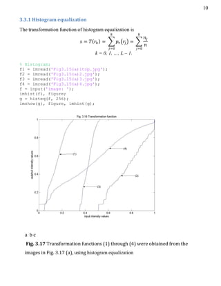
二、 直方圖處理
1. 直方圖等化處理
2. 直方圖匹配處理
三、 使用算術/邏輯運算做增強
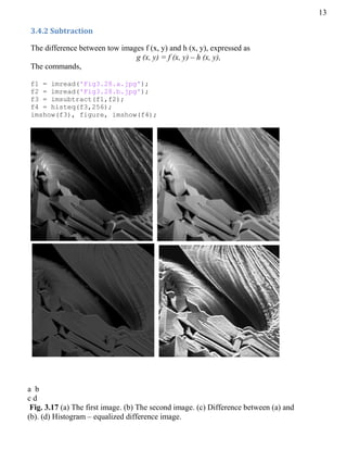
1. 影像相減增強
2. 影像平均增強
四、 平滑空間濾波器
1. 平滑線性濾波器
2. 排序統計濾波器
五、 銳化空間濾波器
1. 拉普拉斯銳化空間濾波器
2. 梯度銳化空間濾波器](https://image.slidesharecdn.com/digital-image-processing-using-matlab-basic-transformations-filters-operators-140529193837-phpapp01/85/Digital-image-processing-using-matlab-basic-transformations-filters-and-operators-3-320.jpg)
![3
SOLUTION
Using Matlab for solving the problem
3.2.1 Negative transformation
Given an image (input image) with gray level in the interval [0, L-1], the negative of that
image is obtained by using the expression: s = (L – 1) – r,
Where r is the gray level of the input image, and s is the gray level of the output.
In Matlab, we use the commands,
>> f=imread('Fig3.04(a).jpg');
g = imcomplement(f);
imshow(f), figure, imshow(g)
In/output image Out/in image
3.2.2 Log transformation
The Logarithm transformations are implemented using the expression:
s = c*log (1+r).
In this case, c = 1. The commands,
>> f=imread('Fig3.05(a).jpg');
g=im2uint8 (mat2gray (log (1+double (f))));
imshow(f), figure, imshow(g)](https://image.slidesharecdn.com/digital-image-processing-using-matlab-basic-transformations-filters-operators-140529193837-phpapp01/85/Digital-image-processing-using-matlab-basic-transformations-filters-and-operators-4-320.jpg)
![4
In/output image Out/in image
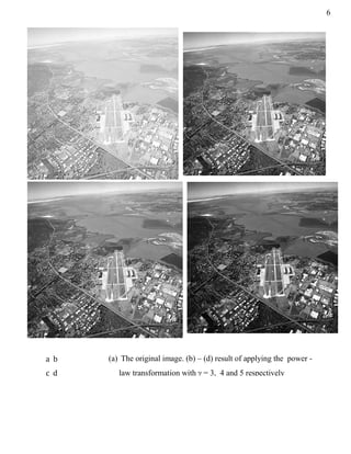
3.2.3 Power-law transformation
Power-law transformations have the basic form,
s = c*r. ^, where c and are positive constants.
The commands,
>> f = imread ('Fig3.08(a).jpg');
f = im2double (f);
[m n]=size (f);
c = 1;
gama = input('gama value = ');
for i=1:m
for j=1:n
g(i,j)=c*(f(i,j)^gama);
end
end;
imshow(f),figure, imshow(g);
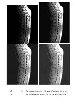
With = 0.6, 0.4 and 0.3 respectively, we can get three images respectively, as shown in the
following figure,](https://image.slidesharecdn.com/digital-image-processing-using-matlab-basic-transformations-filters-operators-140529193837-phpapp01/85/Digital-image-processing-using-matlab-basic-transformations-filters-and-operators-5-320.jpg)
![7
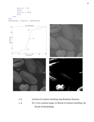
3.2.4 Piecewise-linear transformation
Contrast stretching
The commands,
% function contrast stretching;
>> r1 = 100; s1 = 40;
r2 = 141; s2 = 216;
a = (s1/r1);
b = ((s2-s1)/ (r2-r1));
c = ((255-s2)/ (255-r2));
k = 0:r1;
y1 = a*k;
plot (k,y1); hold on;
k = r1: r2;
y2 = b*(k - r1) + a*r1;
plot (k,y2);
k = r2+1:255;
y3 = c*(k-r2) + b*(r2-r1)+a*r1;
plot (k,y3);
xlim([0 255]);
ylim([0 255]);
xlabel('input gray level, r');
ylabel('outphut gray level, s');
title('Form of transformation');
hold on; figure;
f = imread('Fig3.10(b).jpg');
[m, n] = size (f);
for i = 1:m
for j = 1:n
if((f(i,j)>=0) & (f(i,j)<=r1))
g(i,j) = a*f(i,j);
else
if((f(i,j)>r1) & (f(i,j)<=r2))
g(i,j) = ((b*(f(i,j)-r1)+(a*r1)));
else
if((f(i,j)>r2) & (f(i,j)<=255))
g(i,j) = ((c*(f(i,j)-r2)+(b*(r2-r1)+(a*r1))));
end
end
end
end
end
imshow(f), figure, imshow(g);
% function thresholding
>> f = imread('Fig3.10(b).jpg');
[m, n] = size(f);
for i = 1:m
for j = 1:n
if((f(i,j)>=0) & (f(i,j)<128))](https://image.slidesharecdn.com/digital-image-processing-using-matlab-basic-transformations-filters-operators-140529193837-phpapp01/85/Digital-image-processing-using-matlab-basic-transformations-filters-and-operators-8-320.jpg)
![14
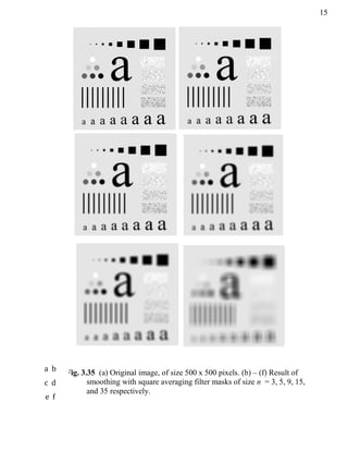
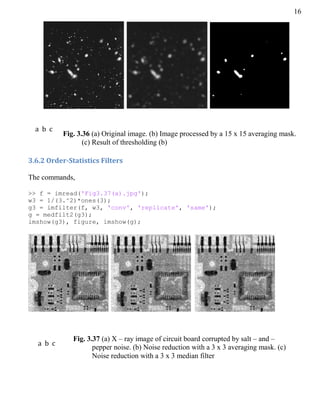
3.6.1 Smoothing Linear Filters
The commands,
f = imread('Fig3.35(a).jpg');
w3 = 1/ (3. ^2)*ones (3);
g3 = imfilter (f, w3, 'conv', 'replicate', 'same');
w5 = 1/ (5. ^2)*ones (5);
g5 = imfilter (f, w5, 'conv', 'replicate', 'same');
w9 = 1/ (9. ^2)*ones (9);
g9 = imfilter (f, w9, 'conv', 'replicate', 'same');
w15 = 1/ (15. ^2)*ones (15);
g15 = imfilter (f, w15, 'conv', 'replicate', 'same');
w35 = 1/ (35. ^2)*ones (35);
g35 = imfilter(f, w35, 'conv', 'replicate', 'same');
imshow (g3), figure, imshow (g5), figure, imshow (g9), figure, imshow
(g15), figure, imshow (g35), figure;
h = imread ('Fig3.36(a).jpg');
h15 = imfilter (h, w15, 'conv', 'replicate', 'same');
[m, n] = size (h15);
for i = 1:m
for j = 1:n
if ((h15 (i,j)>=0) & (h15 (i,j)<128))
g (i,j) = 0;
else
g(i,j) = 255;
end
end
end
imshow(h15), figure, imshow(g);](https://image.slidesharecdn.com/digital-image-processing-using-matlab-basic-transformations-filters-operators-140529193837-phpapp01/85/Digital-image-processing-using-matlab-basic-transformations-filters-and-operators-15-320.jpg)
![17
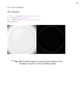
3.7.2 The Laplacian
The Laplacian for image enhancement is as follows:
( )
{
( ) ( )
( ) ( )
( )
The commands,
% Laplacian function
f1 = imread('Fig3.40(a).jpg');
w4 = fspecial('laplacian', 0);
g1 = imfilter(f1, w4, 'replicate');
imshow(g1, [ ]), figure;
f2 = im2double(f1);
g2 = imfilter(f2, w4, 'replicate');
imshow(g2, [ ]), figure;
g3 = imsubtract(f2,g2);
imshow(g3)
Fig. 3.40 (a) Image of
the North Pole
of the moon.
(b) Laplacian
image scaled
for display
purposes. (d)
Image
enhanced by
Eq. (3.7 – 5)
a b
c d](https://image.slidesharecdn.com/digital-image-processing-using-matlab-basic-transformations-filters-operators-140529193837-phpapp01/85/Digital-image-processing-using-matlab-basic-transformations-filters-and-operators-18-320.jpg)
![18
% Laplacian simplication
f1 = imread ('Fig3.41(c).jpg');
w5 = [0 -1 0; -1 5 -1; 0 -1 0];
g1 = imfilter (f1, w5, 'replicate');
imshow (g1), figure;
w9 = [-1 -1 -1; -1 9 -1; -1 -1 -1];
g2 = imfilter (f1, w9, 'replicate');
imshow (g2);
0 -1 0
-1 5 -1
0 -1 0
-1 -1 -1
-1 9 -1
-1 -1 -1
a b c
d e
Fig. 3.37 (a) Composite Laplacian mask. (b) A second composite
mask. (c) Scanning electron microscope image. (d) and (e)
Result of filtering with the masks in (a) and (b) respectively.](https://image.slidesharecdn.com/digital-image-processing-using-matlab-basic-transformations-filters-operators-140529193837-phpapp01/85/Digital-image-processing-using-matlab-basic-transformations-filters-and-operators-19-320.jpg)

This document provides code solutions in Matlab for image processing homework assignments. It includes code to perform: 1. Basic grayscale transformations like negative, log, power-law, and piecewise linear on various images. 2. Histogram processing techniques like equalization and subtraction on images. 3. Smoothing and sharpening filters like averaging, median, Laplacian, and Sobel gradient filters to reduce noise and enhance edges. 4. Detailed explanations and examples are given for each transformation and filtering technique along with input and output images. The code utilizes various Matlab functions to perform the image processing tasks in a concise manner.