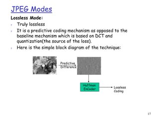
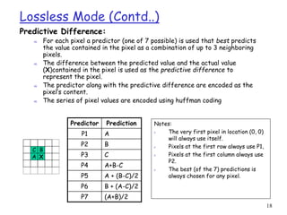
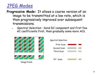
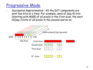
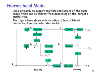
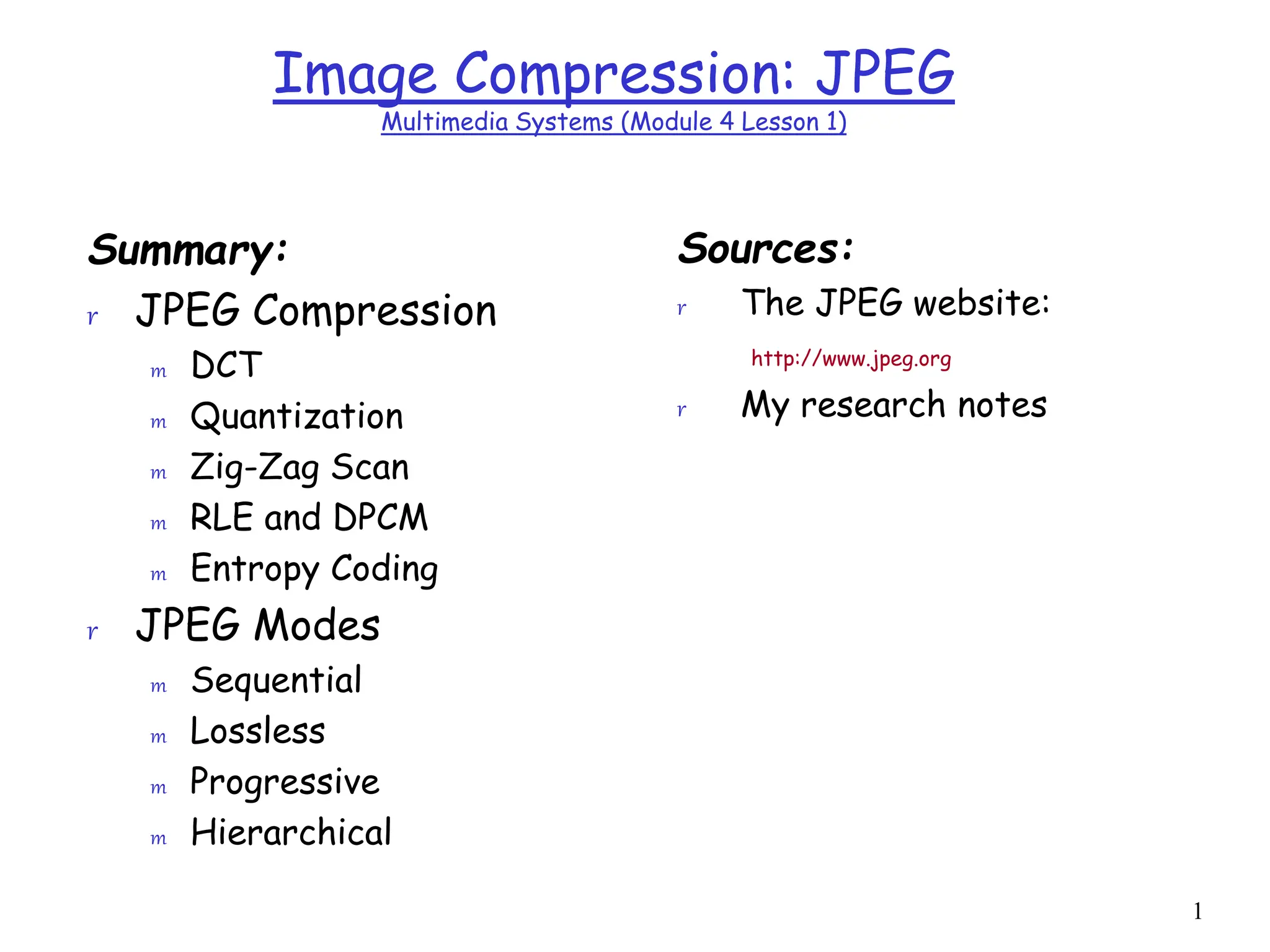
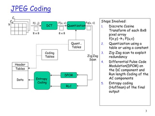
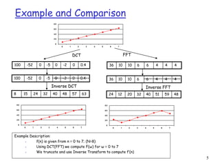
JPEG uses DCT, quantization, and entropy coding to provide lossy compression of images. It can operate in several modes, including sequential, lossless, progressive, and hierarchical. Sequential mode encodes the whole image in a single left-to-right, top-to-bottom scan. Lossless mode uses predictive coding to encode images without loss. Progressive mode transmits an initial coarse version that is progressively improved over multiple transmissions.

1. 1
Image Compression: JPEG
Multimedia Systems (Module 4 Lesson 1)
Summary:
r JPEG Compression
m DCT
m Quantization
m Zig-Zag Scan
m RLE and DPCM
m Entropy Coding
r JPEG Modes
m Sequential
m Lossless
m Progressive
m Hierarchical
Sources:
r The JPEG website:
http://www.jpeg.org
r My research notes

2. 2
Why JPEG
r The compression ratio of lossless methods (e.g.,
Huffman, Arithmetic, LZW) is not high enough for
image and video compression.
r JPEG uses transform coding, it is largely based on
the following observations:
m Observation 1: A large majority of useful image contents
change relatively slowly across images, i.e., it is unusual
for intensity values to alter up and down several times in
a small area, for example, within an 8 x 8 image block.
A translation of this fact into the spatial frequency
domain, implies, generally, lower spatial frequency
components contain more information than the high
frequency components which often correspond to less
useful details and noises.
m Observation 2: Experiments suggest that humans are
more immune to loss of higher spatial frequency
components than loss of lower frequency components.

3. 3
JPEG Coding
Y
Cb
Cr
DPCM
RLC
Entropy
Coding
Header
Tables
Data
Coding
Tables
Quant…
Tables
DCT
f(i, j)
8 x 8
F(u, v)
8 x 8
Quantization
Fq(u, v)
Zig Zag
Scan
Steps Involved:
1. Discrete Cosine
Transform of each 8x8
pixel array
f(x,y) T F(u,v)
2. Quantization using a
table or using a constant
3. Zig-Zag scan to exploit
redundancy
4. Differential Pulse Code
Modulation(DPCM) on
the DC component and
Run length Coding of the
AC components
5. Entropy coding
(Huffman) of the final
output

4. 4
DCT : Discrete Cosine Transform
DCT converts the information contained in a block(8x8) of
pixels from spatial domain to the frequency domain.
m A simple analogy: Consider a unsorted list of 12 numbers
between 0 and 3 -> (2, 3, 1, 2, 2, 0, 1, 1, 0, 1, 0, 0). Consider a
transformation of the list involving two steps (1.) sort the list
(2.) Count the frequency of occurrence of each of the numbers
->(4,4,3,1 ). : Through this transformation we lost the spatial
information but captured the frequency information.
m There are other transformations which retain the spatial
information. E.g., Fourier transform, DCT etc. Therefore
allowing us to move back and forth between spatial and
frequency domains.
1-D DCT: 1-D Inverese DCT:

5. 5
Example and Comparison
0
2 0
4 0
6 0
8 0
0 1 2 3 4 5 6 7
100 -52 0 -5 0 -2 0 0.4 36 10 10 6 6 4 4 4
36 10 10 6 6 4 4 4
100 -52 0 -5 0 -2 0 0.4
24 12 20 32 40 51 59 48
8 15 24 32 40 48 57 63
0
2 0
4 0
6 0
8 0
0 1 2 3 4 5 6 7
0
2 0
4 0
6 0
8 0
0 1 2 3 4 5 6 7
DCT FFT
Inverse DCT Inverse FFT
Example Description:
r f(n) is given from n = 0 to 7; (N=8)
r Using DCT(FFT) we compute F(ω) for ω = 0 to 7
r We truncate and use Inverse Transform to compute f’(n)

6. 6
2-D DCT
r Images are two-dimensional; How do you perform 2-D DCT?
m Two series of 1-D transforms result in a 2-D transform as
demonstrated in the figure below
1-D
Row-
wise
1-D
Column-
wise
8x8 8x8 8x8
j)
f(i,
v)
F(u,
r F(0,0) is called the DC component and the rest of F(i,j) are called
AC components

7. 7
2-D Transform Example
r The following example will demonstrate the idea behind a 2-
D transform by using our own cooked up transform: The
transform computes a running cumulative sum.
1
1-D
Row-
wise
1-D
Column-
wise
8x8
8x8
8x8
1
1
1
1
1
1
1
1
1
1
1
1
1
1
1
1
1
1
1
1
1
1
1
1
1
1
1
1
1
1
1
1
1
1
1
1
1
1
1
1
1
1
1
1
1
1
1
1
1
1
1
1
1
1
1
1
1
1
1
1
1
1
1
8 7 6 5 4 3 2 1
8 7 6 5 4 3 2 1
8 7 6 5 4 3 2 1
8 7 6 5 4 3 2 1
8 7 6 5 4 3 2 1
8 7 6 5 4 3 2 1
8 7 6 5 4 3 2 1
8 7 6 5 4 3 2 1
64 56 48 40 32 24 16 8
56
48
40
32
24
16
8
49
42
35
28
21
14
7
42
36
30
24
18
12
6
35
30
25
20
15
10
5
28
24
20
16
12
8
4
21
18
15
12
9
6
3
14
12
10
8
6
4
2
7
6
5
4
3
2
1
 

8
n
my (n)
f
)
(
F 

My Transform:
j)
f(i,
v)
(u,
my
F
Note that this is only a hypothetical
transform. Do not confuse this with DCT

8. 8
Quantization
r Why? -- To reduce number of bits per sample
F’(u,v) = round(F(u,v)/q(u,v))
r Example: 101101 = 45 (6 bits).
Truncate to 4 bits: 1011 = 11. (Compare 11 x 4 =44 against 45)
Truncate to 3 bits: 101 = 5. (Compare 8 x 5 =40 against 45)
Note, that the more bits we truncate the more precision we lose
r Quantization error is the main source of the Lossy
Compression.
r Uniform Quantization:
m q(u,v) is a constant.
r Non-uniform Quantization -- Quantization Tables
m Eye is most sensitive to low frequencies (upper left corner in
frequency matrix), less sensitive to high frequencies (lower right
corner)
m Custom quantization tables can be put in image/scan header.
m JPEG Standard defines two default quantization tables, one
each for luminance and chrominance.

9. 9
Zig-Zag Scan
r Why? -- to group low frequency coefficients in top of vector
and high frequency coefficients at the bottom
r Maps 8 x 8 matrix to a 1 x 64 vector
8x8
. . .
1x64

10. 10
DPCM on DC Components
r The DC component value in each 8x8 block is large and varies
across blocks, but is often close to that in the previous block.
r Differential Pulse Code Modulation (DPCM): Encode the
difference between the current and previous 8x8 block.
Remember, smaller number -> fewer bits
45
54
48
32
45
9
-6
12
36 4
.
.
.
.
.
.
1x64
1x64
1x64
1x64
1x64
1x64
1x64
1x64
1x64
1x64

11. 11
RLE on AC Components
r The 1x64 vectors have a lot of zeros in them, more so towards
the end of the vector.
m Higher up entries in the vector capture higher frequency (DCT)
components which tend to be capture less of the content.
m Could have been as a result of using a quantization table
r Encode a series of 0s as a (skip,value) pair, where skip is the
number of zeros and value is the next non-zero component.
m Send (0,0) as end-of-block sentinel value.
. . .
1x64
0 0 0 0 0 1 1 0 0 0 0 0
5,1
0 0
7,2
0 . . .
2

12. 12
Entropy Coding: DC Components
SIZE Value Code
0 0 ---
1 -1,1 0,1
2 -3, -2, 2,3 00,01,10,11
3 -7,…, -4, 4,…, 7 000,…, 011, 100,…111
4 -15,…, -8, 8,…, 15 0000,…, 0111, 1000,…, 1111
. .
. .
11 -2047,…, -1024, 1024,… 2047 …
r DC components are differentially coded as (SIZE,Value)
m The code for a Value is derived from the following table
Size_and_Value Table

13. 13
Entropy Coding: DC Components (Contd..)
SIZE Code
Length
Code
0 2 00
1 3 010
2 3 011
3 3 100
4 3 101
5 3 110
6 4 1110
7 5 11110
8 6 111110
9 7 1111110
10 8 11111110
11 9 111111110
r DC components are differentially coded as (SIZE,Value)
m The code for a SIZE is derived from the following table
Example: If a DC component is 40
and the previous DC
component is 48. The
difference is -8. Therefore it
is coded as:
1010111
0111: The value for representing –8
(see Size_and_Value table)
101: The size from the same table
reads 4. The corresponding
code from the table at left is
101.
Huffman Table for DC component SIZE field

14. 14
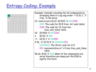
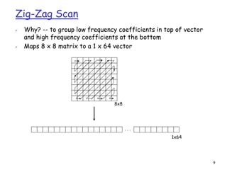
Entropy Coding: AC Components
r AC components (range –1023..1023) are coded as (S1,S2 pairs):
m S1: (RunLength/SIZE)
• RunLength: The length of the consecutive zero values [0..15]
• SIZE: The number of bits needed to code the next nonzero AC component’s value. [0-A]
• (0,0) is the End_Of_Block for the 8x8 block.
• S1 is Huffman coded (see AC code table below)
m S2: (Value)
• Value: Is the value of the AC component.(refer to size_and_value table)
Run/
SIZE
Code
Length
Code
0/0 4 1010
0/1 2 00
0/2 2 01
0/3 3 100
0/4 4 1011
0/5 5 11010
0/6 7 1111000
0/7 8 11111000
0/8 10 1111110110
0/9 16 1111111110000010
0/A 16 1111111110000011
Run/
SIZE
Code
Length
Code
1/1 4 1100
1/2 5 11011
1/3 7 1111001
1/4 9 111110110
1/5 11 11111110110
1/6 16 1111111110000100
1/7 16 1111111110000101
1/8 16 1111111110000110
1/9 16 1111111110000111
1/A 16 1111111110001000
… 15/A More Such rows

15. 15
Entropy Coding: Example
Example: Consider encoding the AC components by
arranging them in a zig-zag order -> 12,10, 1, -7
2 0s, -4, 56 zeros
12: read as zero 0s,12: (0/4)12  10111100
1011: The code for (0/4 from AC code table)
1100: The code for 12 from the
Size_and_Value table.
10: (0/4)10  10111010
1: (0/1)1  001
-7: (0/3)-7  100000
2 0s, -4: (2/3)-4  1111110111011
1111110111: The 10-bit code for 2/3
011: representation of –4 from Size_and_Value
table.
56 0s: (0,0)  1010 (Rest of the components are
zeros therefore we simply put the EOB to
signify this fact)
40 12 0 0 0 0 0 0
10 -7 -4 0 0 0 0 0
1 0 0 0 0 0 0 0
0 0 0 0 0 0 0 0
0 0 0 0 0 0 0 0
0 0 0 0 0 0 0 0
0 0 0 0 0 0 0 0
0 0 0 0 0 0 0 0

16. 16
JPEG Modes
Sequential Mode:
r Each image is encoded in a single left-to-right,
top-to-bottom scan.
m The technique we have been discussing so far is an
example of such a mode, also referred to as the Baseline
Sequential Mode.
m It supports only 8-bit images as opposed to 12-bit images
as described before.

17. 17
JPEG Modes
Lossless Mode:
r Truly lossless
r It is a predictive coding mechanism as opposed to the
baseline mechanism which is based on DCT and
quantization(the source of the loss).
r Here is the simple block diagram of the technique:
Predictive
Difference
Huffman
EnCoder
Lossless
Coding

18. 18
Lossless Mode (Contd..)
Predictive Difference:
m For each pixel a predictor (one of 7 possible) is used that best predicts
the value contained in the pixel as a combination of up to 3 neighboring
pixels.
m The difference between the predicted value and the actual value
(X)contained in the pixel is used as the predictive difference to
represent the pixel.
m The predictor along with the predictive difference are encoded as the
pixel’s content.
m The series of pixel values are encoded using huffman coding
C B
A X
Predictor Prediction
P1 A
P2 B
P3 C
P4 A+B-C
P5 A + (B-C)/2
P6 B + (A-C)/2
P7 (A+B)/2
Notes:
r The very first pixel in location (0, 0)
will always use itself.
r Pixels at the first row always use P1,
r Pixels at the first column always use
P2.
r The best (of the 7) predictions is
always chosen for any pixel.

19. 19
JPEG Modes
Progressive Mode: It allows a coarse version of an
image to be transmitted at a low rate, which is
then progressively improved over subsequent
transmissions.
m Spectral Selection : Send DC component and first few
AC coefficients first, then gradually some more ACs.
Spectral Selection:
First Scan:
Second Scan:
Third Scan:
.
.
Nth Scan:
Image Pixels

20. 20
Progressive Mode
r Successive Approximation : All the DCT components are
sent few bits at a time: For example, send n1 (say,4) bits
(starting with MSB) of all pixels in the first scan, the next
n2(say 1) bits of all pixels in the second and so on.
Pixels ordered (zig-zag-wise)
First Scan:
Second Scan:
Third Scan:
5th Scan:
7 6 5 4 0
3 2 1
MSB LSB
.
.
. . .
. . .
. . .
. . .
.
.
One Pixel

21. 21
Hierarchical Mode
r Used primarily to support multiple resolutions of the same
image which can be chosen from depending on the target’s
capabilities.
r The figure here shows a description of how a 3-level
hierarchical encoder/decoder works:
2x2 Encode
Decode
4x4 Encode
Decode
2x2
2x2
+
-
+ +
+
-
L4
L2
L1
I
Encode
Decode
Decode
Decode
Decoding
Encoding
4x4
2x2
2x2
+
+
I4
I2
I’4
I’2
I’