Chapter 1 - Introduction

ECE 285
Machine Learning for Image Processing
Chapter I – Introduction
Charles Deledalle
March 29, 2019
(Source: Jeﬀ Walsh)
1

Who?
Who am I?
• A visiting scholar from University of Bordeaux (France).
• Visiting UCSD since Jan 2017.
• PhD in signal processing (2011).
• Research in image processing / applied maths.
• Aﬃliated with CNRS (French scientiﬁc research institute).
• Email: cdeledalle@ucsd.edu
• www.charles-deledalle.fr
2

What?
What is it about?
Machine learning / Deep learning
applied to
Image processing / Computer vision
• A bit of theory (but not exhaustive), a bit of math (but not too much),
• Mainly: concepts, vocabulary, recent successful models and applications.
3

What?
What is it about? – Two examples
(Source: Luc et al., 2017) (Karpathy & Fei-Fei, 2015)
(CV:) Automatic extraction of high level information from images/videos,
(ML:) by learning from tons of (annotated) examples.
4

What?
What is it about? – A multidisciplinary ﬁeld
5

What? Syllabus
• Introduction to image sciences and machine learning
• Examples of image processing and computer vision tasks,
• Overview of learning problems, approaches and workflow.
• Preliminaries to deep learning
• Perceptron, Artificial Neural Networks (NNs),
• Backpropagation, Support Vector Machines.
• Basics of deep learning
• Representation learning, auto-encoders, algorithmic recipes.
• Applications
• Image classification
• Image generation
• Object detection
• Super resolution
• Image captioning
• Style transfer
⇒ Convolutional NNs, Recurrent NNs, Generative adversarial networks.
• Labs and project using Python & PyTorch.
6

Why?
Why machine learning / deep learning?
• In the past 10 years, machine learning and artiﬁcial
intelligence have shown tremendous progress.
• The recent success can be attributed to:
• Explosion of data,
• Cheap computing cost – CPUs and GPUs,
• Improvements of machine learning models.
• Much of the current excitement concerns a subﬁeld of
it called “deep learning”.
(Source: Poo Kuan Hoong)
Googletrends
7

Why?
Why image processing / computer vision?
• Images become a major communication media.
• Image data need to be analyzed automatically
• Reduce the burden of human operators by
teaching a computer to see.
• To produce images with artistic eﬀect.
• Many applications: robotic, medical, video games,
sport, smart cars, . . .
8

Why?
Why? More examples. . .
(Source: Stanford 2017’CS231n class) 9

What for?
What for?
• Industry: be able to use or implement latest machine learning techniques
to solve image processing and computer vision tasks.
• Big actors: Amazon, Google, Microsoft, Facebook, . . .
10

What for?
What for?
• Academic: be able to read and understand latest research papers, and
possibly publish new ones.
• Big actors: Stanford, New York U., U. of Montreal, U. of Toronto, . . .
• Main conferences: NIPS, CVPR, ICML, . . .
11

How?
How? – Teaching staﬀ
Instructor
Charles Deledalle
Teaching assistants
Sneha Gupta Abhilash Kasarla Anurag Paul Inderjot
Singh Saggu
12

How?
How? – Schedule
• 30× 50 min lectures (10 weeks)
• Mon/Wed/Fri 3:00-3:50pm
• Room CENTR 115
• 5× 2 hour optional labs every two weeks (refer to Google’s calendar)
• Group 1: Fri 10am-12pm (lastnames from A to Kan)
• Group 2: Tues 2-4pm (lastnames from Kar to Ra)
• Group 3: Thurs 2-4pm (lastnames from Ro to Z)
• Jacobs Hall, Room 4309
Please, coordinate with your classmates to switch groups.
• Oﬃce hours
• Charles Deledalle, Weekly on Tues 10am-12pm, Jacobs Hall 4808.
• TAs, every two other weeks, TBA
• Google calendar: https://tinyurl.com/y2gltvzs
13

How?
How? – Assignments / Project / Evaluation
• 4 assignments in Python/Pytorch (individual) . . . . . . . . . . . . . . . . . . . 40%
• Don’t wait for the lectures to start,
• You can start doing them all now.
• 1 project open-ended or to choose among 3 proposed subjects . . . . 30%
• In groups of 3 or 4 (start looking for a group now),
• Details to be announced in a couple of weeks.
• 3 quizzes (∼45 mins each) . . . . . . . . . . . . . . . . . . . . . . . . . . . . . . . . . . . . . . 30%
• Multiple choice on the topics of all previous lectures,
• Dates are: April 24, May 17, June 10 (3-3:50pm, CENTR 115)
• No documents allowed.
14

How?
How? – What assignments?
Assignment 1 (Backpropagation): Create form scratch a simple machine
learning technique to recognize hand-written digits from 0 to 9.
−→ 96% success
Assignment 2 (CNNs and PyTorch): Develop a deep learning technique and
learn how to use GPUs with PyTorch.
Improve your results to 98%!
15

How?
Assignment 3 (Transfer learning): Teach a program how to recognize bird
species when only a small dataset is available.
−→ Mocking bird!
16

How?
Assignment 4 (Image Denoising): Teach a program how to remove noise.
−→
17

How?
How? – Assignments and Project Deadlines
Calendar Deadline
1 Assignment 0 – Python/Numpy/Matplotlib (Prereq) . . . . . . . . . . . . . . . . optional
2 Assignment 1 – Backpropagation . . . . . . . . . . . . . . . . . . . . . . . . . . . . . . . . . . . April 17
3 Assignment 2 – CNNs and PyTorch . . . . . . . . . . . . . . . . . . . . . . . . . . . . . . . . . . May 1
4 Assignment 3 – Transfer Learning . . . . . . . . . . . . . . . . . . . . . . . . . . . . . . . . . . . May 15
5 Assignment 4 – Image Denoising . . . . . . . . . . . . . . . . . . . . . . . . . . . . . . . . . . . . May 29
6 Project . . . . . . . . . . . . . . . . . . . . . . . . . . . . . . . . . . . . . . . . . . . . . . . . . . . . . . . . . . . . . June 7
Refer to the Google calendar: https://tinyurl.com/y2gltvzs
18

How?
How? – Prerequisites
• Linear algebra + Differential calculus + Basics of optimization + Statistics/Probabilities
• Python programming (at least Assignment 0)
Optional: cookbook for data scientists
Cookbook for data scientists
Charles Deledalle
Convex optimization
Conjugate gradient
Let A ∈ Cn×n
be Hermitian positive definite The
sequence xk defined as, r0 = p0 = b, and
xk+1 = xk + αkpk
rk+1 = rk − αkApk
with αk =
r∗
krk
p∗
kApk
pk+1 = rk+1 + βkpk with βk =
r∗
k+1rk+1
r∗
krk
converges towards A−1
b in at most n steps.
Lipschitz gradient
f : Rn
→ R has a L Lipschitz gradient if
|| f(x) − f(y)||2 L||x − y||2
If f(x) = Ax, L = ||A||2. If f is twice differentiable
L = supx ||Hf (x)||2, i.e., the highest eigenvalue of
Hf (x) among all possible x.
Convexity
f : Rn
→ R is convex if for all x, y and λ ∈ (0, 1)
f(λx + (1 − λ)y) λf(x) + (1 − λ)f(y)
f is strictly convex if the inequality is strict. f is
convex and twice differentiable iif Hf (x) is Hermitian
non-negative definite. f is strictly convex and twice
differentiable iif Hf (x) is Hermitian positive definite.
If f is convex, f has only global minima if any. We
write the set of minima as
argmin
x
f(x) = {x for all z ∈ Rn
f(x) f(z)}
Gradient descent
Let f : Rn
→ R be differentiable with L Lipschitz
gradient then, for 0 < γ 1/L, the sequence
xk+1 = xk − γ f(xk)
converges towards a stationary point x in O(1/k)
f(x ) = 0
If f is moreover convex then
x ∈ argmin
x
f(x).
Newton’s method
Let f : Rn
→ R be convex and twice continuously
differentiable then, the sequence
xk+1 = xk − Hf (xk)−1
f(xk)
converges towards a minimizer of f in O(1/k2
).
Subdifferential / subgradient
The subdifferential of a convex†
function f is
∂f(x) = {p ∀x , f(x) − f(x ) p, x − x } .
p ∈ ∂f(x) is called a subgradient of f at x.
A point x is a global minimizer of f iif
0 ∈ ∂f(x ).
If f is differentiable then ∂f(x) = { f(x)}.
Proximal gradient method
Let f = g + h with g convex and differentiable with
Lip. gradient and h convex†
. Then, for 0<γ 1/L,
xk+1 = proxγh(xk − γ g(xk))
converges towards a global minimizer of f where
proxγh(x) = (Id + γ∂h)−1
(x)
= argmin
z
1
2
||x − z||2
+ γh(z)
is called proximal operator of f.
Convex conjugate and primal dual problem
The convex conjugate of a function f : Rn
→ R is
f∗
(z) = sup
x
z, x − f(x)
if f is convex (and lower semi-continuous) f = f .
Moreover, if f(x) = g(x) + h(Lx), then minimizers
x of f are solutions of the saddle point problem
(x , z ) ∈ args min
x
max
z
g(x) + Lx, z − h∗
(z)
z is called dual of x and satisfies
Lx ∈ ∂h∗
(z )
L∗
z ∈ ∂g(x )
Charles Deledalle
Multi-variate differential calculus
Partial and directional derivatives
Let f : Rn
→ Rm
. The (i, j)-th partial derivative of
f, if it exists, is
∂fi
∂xj
(x) = lim
ε→0
fi(x + εej) − fi(x)
ε
where ei ∈ Rn
, (ej)j = 1 and (ej)k = 0 for k = j.
The directional derivative in the dir. d ∈ Rn
is
Ddf(x) = lim
ε→0
f(x + εd) − f(x)
ε
∈ Rm
Jacobian and total derivative
Jf =
∂f
∂x
=
∂fi
∂xj i,j
(m × n Jacobian matrix)
df(x) = tr
∂f
∂x
(x) dx (total derivative)
Gradient, Hessian, divergence, Laplacian
f =
∂f
∂xi i
(Gradient)
Hf = f =
∂2
f
∂xi∂xj i,j
(Hessian)
div f = t
f =
n
i=1
∂fi
∂xi
= tr Jf (Divergence)
∆f = div f =
n
i=1
∂2
f
∂x2
i
= tr Hf (Laplacian)
Properties and generalizations
f = Jt
f (Jacobian ↔ gradient)
div = − ∗
(Integration by part)
df(x) = tr [Jf dx] (Jacob. character. I)
Ddf(x) = Jf (x) × d (II)
f(x+h)=f(x) + Dhf(x) + o(||h||) (1st order exp.)
f(x+h)=f(x) + Dhf(x) + 1
2h∗
Hf (x)h + o(||h||2
)
∂(f ◦ g)
∂x
=
∂f
∂x
◦ g
∂g
∂x
(Chain rule)
Elementary calculation rules
dA = 0
d[aX + bY ] = adX + bdY (Linearity)
d[XY ] = (dX)Y + X(dY ) (Product rule)
d[X∗
] = (dX)∗
d[X−1
] = −X−1
(dX)X−1
d tr[X] = tr[dX]
dZ
dX
=
dZ
dY
dY
dX
(Leibniz’s chain rule)
Classical identities
d tr[AXB] = tr[BA dX]
d tr[X∗
AX] = tr[X∗
(A∗
+ A) dX]
d tr[X−1
A] = tr[−X−1
AX−1
dX]
d tr[Xn
] = tr[nXn−1
dX]
d tr[eX
] = tr[eX
dX]
d|AXB| = tr[|AXB|X−1
dX]
d|X∗
AX| = tr[2|X∗
AX|X−1
dX]
d|Xn
| = tr[n|Xn
|X−1
dX]
d log |aX| = tr[X−1
dX]
d log |X∗
X| = tr[2X+
dX]
Implicit function theorem
Let f : Rn+m
→ Rn
be continuously differentiable
and f(a, b) = 0 for a ∈ Rn
and b ∈ Rm
. If ∂f
∂y (a, b)
is invertible, then there exist g such that g(a) = b
and for all x ∈ Rn
in the neighborhood of a
f(x, g(x)) = 0
∂g
∂xi
(x) = −
∂f
∂y
(x, g(x))
−1
∂f
∂xi
(x, g(x))
In a system of equations f(x, y) = 0 with an infinite
number of solutions (x, y), IFT tells us about the
relative variations of x with respect to y, even in
situations where we cannot write down explicit
solutions (i.e., y = g(x)). For instance, without
solving the system, it shows that the solutions (x, y)
of x2
+ y2
= 1 satisfies ∂y
∂x = −x/y.
Charles Deledalle
Probability and Statistics
Kolmogorov’s probability axioms
Let Ω be a sample set and A an event
P[Ω] = 1, P[A] 0
P
∞
i=1
Ai =
∞
i=1
P[Ai] with Ai ∩ Aj = ∅
Basic properties
P[∅] = 0, P[A] ∈ [0, 1], P[Ac
] = 1 − P[A]
P[A] P[B] if A ⊆ B
P[A ∪ B] = P[A] + P[B] − P[A ∩ B]
Conditional probability
P[A|B] =
P[A ∩ B]
P[B]
subject to P[B] > 0
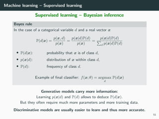
Bayes’ rule
P[A|B] =
P[B|A]P[A]
P[B]
Independence
Let A and B be two events, X and Y be two rv
A⊥B if P[A ∩ B] = P[A]P[B]
X⊥Y if (X x)⊥(Y y)
If X and Y admit a density, then
X⊥Y if fX,Y (x, y) = fX(x)fY (y)
Properties of Independence and uncorrelation
P[A|B] = P[A] ⇒ A⊥B
X⊥Y ⇒ (E[XY ∗
] = E[X]E[Y ∗
] ⇔ Cov[X, Y ] = 0)
Independence ⇒ uncorrelation
correlation ⇒ dependence
uncorrelation Independence
dependence correlation
Discrete random vectors
Let X be a discrete random vector defined on Nn
E[X]i =
∞
k=0
kP[Xi = k]
The function fX : k → P[X = k] is called the
probability mass function (pmf) of X.
Continuous random vectors
Let X be a continuous random vector on Cn
.
Assume there exist fX such that, for all A ⊆ Cn
,
P[X ∈ A] =
A
fX(x) dx.
Then fX is called the probability density function
(pdf) of X, and
E[X] =
Cn
xfX(x) dx.
Variance / Covariance
Let X and Y be two random vectors. The
covariance matrix between X and Y is defined as
Cov[X, Y ] = E[XY ∗
] − E[X]E[Y ]∗
.
X and Y are said uncorrelated if Cov[X, Y ] = 0.
The variance-covariance matrix is
Var[X] = Cov[X, X] = E[XX∗
] − E[X]E[X]∗
.
Basic properties
• The expectation is linear
E[aX + bY + c] = aE[X] + bE[Y ] + c
• If X and Y are independent
Var[aX + bY + c] = a2
Var[X] + b2
Var[Y ]
• Var[X] is always Hermitian positive definite
Charles Deledalle
Fourier analysis
Fourier Transform (FT)
Let x : R → C such that
+∞
−∞
|x(t)| dt < ∞. Its
Fourier transform X : R → C is defined as
X(u) = F[x](u) =
+∞
−∞
x(t)e−i2πut
dt
x(t) = F−1
[X](t) =
+∞
−∞
X(u)ei2πut
du
where u is referred to as the frequency.
Properties of continuous FT
F[ax + by] = aF[x] + bF[y] (Linearity)
F[x(t − a)] = e−i2πau
F[x] (Shift)
F[x(at)](u) =
1
|a|
F[x](u/a) (Modulation)
F[x∗
](u) = F[x](−u)∗
(Conjugation)
F[x](0) =
+∞
−∞
x(t) dt (Integration)
+∞
−∞
|x(t)|2
dt =
+∞
−∞
|X(u)|2
du (Parseval)
F[x(n)
](u) = (2πiu)n
F[x](u) (Derivation)
F[e−π2at2
](u) =
1
√
πa
e−u2/a
(Gaussian)
x is real ⇔ X(ε) = X(−ε)∗
(Real ↔ Hermitian)
Properties with convolutions
(x y)(t) =
∞
−∞
x(s)y(t − s) ds (Convolution)
F[x y] = F[x]F[y] (Convolution theorem)
Multidimensional Fourier Transform
Fourier transform is separable over the different d
dimensions, hence can be defined recursively as
F[x] = (F1 ◦ F2 ◦ . . . ◦ Fd)[x]
where Fk[x](t1 . . . , εk, . . . , td) =
F[tk → x(t1, . . . , tk, . . . , td)](εk)
and inherits from above properties (same for DFT).
Discrete Fourier Transform (DFT)
Xu = F[x]u =
n−1
t=0
xte−i2πut/n
xt = F−1
[X]t =
1
n
n−1
u=0
Xkei2πut/n
Or in a matrix-vector form X = Fx and x = F−1
X
where Fu,k = e−i2πuk/n
. We have
F∗
= nF−1
and U = n−1/2
F is unitary
Properties of discrete FT
F[ax + by] = aF[x] + bF[y] (Linearity)
F[xt−a] = e−i2πau/n
F[x] (Shift)
F[x∗
]u = F[x]∗
n−u mod n (Conjugation)
F[x]0 =
n−1
t=0
xt (Integration)
||x||2
2 =
1
n
||X||2
2 (Parseval)
||x||1 ||X||1 n||x||1
||X||∞ ||x||1 and ||x||∞
1
n
||X||1
x is real ⇔ Xu = X∗
n−u mod n (Real ↔ Hermitian)
Discrete circular convolution
(x ∗ y)t =
n
s=1
xsy(t−s mod n)+1 or x ∗ y = Φyx
where (Φy)t,s = y(t−s mod n)+1 is a circulant matrix
diagonalizable in the discrete Fourier basis, thus
F[x ∗ y]u = F[x]uF[y]u
Fast Fourier Transform (FFT)
The matrix-by-vector product Fx can be computed
in O(n log n) operations (much faster than the
general matrix-by-vector product that required O(n2
)
operations). Same for F−1
and same for
multi-dimensional signals.
Charles Deledalle
Linear algebra II
Eigenvalues / eigenvectors
If λ ∈ C and e ∈ Cn
(= 0) satisfy
Ae = λe
λ is called the eigenvalue associated to the
eigenvector e of A. There are at most n distinct
eigenvalues λi and at least n linearly independent
eigenvectors ei (with norm 1). The set λi of n (non
necessarily distinct) eigenvalues is called the
spectrum of A (for a proper definition see
characteristic polynomial, multiplicity, eigenspace).
This set has exactly r = rank A non zero values.
Eigendecomposition (m = n)
If it exists E ∈ Cn×n
, and a diagonal matrix
Λ ∈ Cn×n
st
A = EΛE−1
A is said diagonalizable and the columns of E are
the n eigenvectors ei of A with corresponding
eigenvalues Λi,i = λi.
Properties of eigendecomposition (m = n)
• If, for all i, Λi,i = 0, then A is invertible and
A−1
= EΛ−1
E−1
with Λ−1
i,i = (Λi,i)−1
• If A is Hermitian (A = A∗
), such decomposition
always exists, the eigenvectors of E can be chosen
orthonormal such that E is unitary (E−1
= E∗
), and
λi are real.
• If A is Hermitian (A = A∗
) and λi > 0, A is said
positive definite, and for all x = 0, xAx∗
> 0.
Singular value decomposition (SVD)
For all matrices A there exists two unitary matrices
U ∈ Cm×m
and V ∈ Cn×n
, and a real non-negative
diagonal matrix Σ ∈ Rm×n
st
A = UΣV ∗
and A =
r
k=1
σkukv∗
k
with r = rank A non zero singular values Σk,k =σk.
Eigendecomposition and SVD
• If A is Hermitian, the two decompositions coincide
with V = U = E and Σ = Λ.
• Let A = UΣV ∗
be the SVD of A, then the
eigendecomposition of AA∗
is E = U and Λ = Σ2
.
SVD, image and kernel
Let A = UΣV ∗
be the SVD of A, and assume Σi,i
are ordered in decreasing order then
Im[A] = Span({ui ∈ Rm
i ∈ (1 . . . r)})
Ker[A] = Span({vi ∈ Rn
i ∈ (r + 1 . . . n)})
Moore-Penrose pseudo-inverse
The Moore-Penrose pseudo-inverse reads
A+
= V Σ+
U∗
with Σ+
i,i =
(Σi,i)−1
if Σii > 0,
0 otherwise
and is the unique matrix satisfying A+
AA+
= A+
and AA+
A = A with A+
A and AA+
Hermitian.
If A is invertible, A+
= A−1
.
Matrix norms
||A||p = sup
x;||x||p=1
||Ax||p, ||A||2 = max
k
σk, ||A||∗ =
k
σk,
||A||2
F =
i,j
|ai,j|2
= tr A∗
A =
k
σ2
k
Charles Deledalle
Linear algebra I
Notations
x, y, z, . . . : vectors of Cn
a, b, c, . . . : scalars of C
A, B, C : matrices of Cm×n
Id : identity matrix
i = 1, . . . , m and j = 1, . . . , n
Matrix vector product
(Ax)i =
n
k=1
Ai,kxk
(AB)i,j =
n
k=1
Ai,kBk,j
Basic properties
A(ax + by) = aAx + bAy
AId = IdA = A
Inverse (m = n)
A is said invertible, if it exists B st
AB = BA = Id.
B is unique and called inverse of A.
We write B = A−1
.
Adjoint and transpose
(At
)j,i = Ai,j, At
∈ Cm×n
(A∗
)j,i = (Ai,j)∗
, A∗
∈ Cm×n
Ax, y = x, A∗
y
Trace and determinant (m = n)
tr A=
n
i=1
Ai,i =
n
i=1
λi
det A =
n
i=1
λi
tr A = tr A∗
tr AB = tr BA
det A∗
= det A
det A−1
= (det A)−1
det AB = det A det B
A is invertible ⇔ detA = 0 ⇔ λi = 0, ∀i
Scalar products, angles and norms
x, y = x · y = x∗
y =
n
k=1
xkyk (dot product)
||x||2
= x, x =
n
k=1
x2
k ( 2 norm)
| x, y | ||x||||y|| (Cauchy-Schwartz inequality)
cos(∠(x, y)) =
x, y
||x||||y||
(angle and cosine)
||x + y||2
= ||x||2
+ ||y||2
+ 2 x, y (law of cosines)
||x||p
p =
n
k=1
|xk|p
, p 1 ( p norm)
||x + y||p ||x||p + ||y||p (triangular inequality)
Orthogonality, vector space, basis, dimension
x⊥y ⇔ x, y = 0 (Orthogonality)
x⊥y ⇔ ||x + y||2
= ||x||2
+ ||y||2
(Pythagorean)
Let d vectors xi be st xi⊥xj, ||xi|| = 1. Define
V = Span({xi}) = y ∃α ∈ Cd
, y =
d
i=1
αixi
V is a vector space, {xi} is an orthonormal basis of V and
∀y ∈ V, y =
d
i=1
y, xi xi
and d = dim V is called the dimensionality of V . We have
dim(V ∪ W) = dim V + dim W − dim(V ∩ W)
Column/Range/Image and Kernel/Null spaces
Im[A] = {y ∈ Rm
∃x ∈ Rn
such that y = Ax} (image)
Ker[A] = {x ∈ Rn
Ax = 0} (kernel)
Im[A] and Ker[A] are vector spaces satisfying
Im[A] = Ker[A∗
]⊥
and Ker[A] = Im[A∗
]⊥
rank A + dim(Ker[A]) = n (rank-nullity theorem)
where rank A = dim(Im[A]) (matrix rank)
Note also rank A = rank A∗
rank A + dim(Ker[A∗
]) = m
www.charles-alban.fr/pages/teaching/
19

How?
How? – Piazza
https://piazza.com/ucsd/spring2019/ece285mlip
If you cannot get access to it contact me asap
at cdeledalle@ucsd.edu
(title: “[ECE285-MLIP][Piazza] Access issues”).
20

Misc
Misc
Programming environment: Python/PyTorch/Jupyter
• We will use UCSD’s DSML cluster with GPU/CUDA. Great but busy.
• We recommend you to install Conda/Python 3/Jupyter on your laptop.
• Please refer to additional documentations on Piazza.
Communication:
• All your emails must have a title starting with “[ECE285-MLIP]”
→ or it will end up in my spam/trash.
Note: “[ECE 285-MLIP]”, “[ece285 MLIP]”, “(ECE285MLIP)” are invalid!
• But avoid emails, use Piazza to communicate instead.
• For questions that may interest everyone else, post on Piazza forums.
21

Some references
Reference books
C. Bishop
Pattern recognition and Machine Learning
Springer, 2006
T. Hastie, R. Tibshirani, J. Friedman
The Elements of Statistical Learning: Data Mining, Inference, and Prediction
Springer, 2009
http://web.stanford.edu/~hastie/ElemStatLearn/
D. Barber
Bayesian Reasoning and Machine Learning
Cambridge University Press, 2012
http://www.cs.ucl.ac.uk/staff/d.barber/brml/
I. Goodfellow, Y. Bengio and A. Courville.
Deep Learning
MIT Press book, 2017
http://www.deeplearningbook.org/
22

Some references
Reference online classes
Fei-Fei Li, Justin Johnson and Serena Yeung, 2017 (Stanford)
CS231n: Convolutional Neural Networks for Visual Recognition
http://cs231n.stanford.edu
Giró et al, 2017 (Catalonia)
Deep Learning for Artificial Intelligence
https://telecombcn-dl.github.io/2017-dlai/
Leonardo Araujo dos Santos.
Artificial Inteligence
https://www.gitbook.com/@leonardoaraujosantos
23

Imaging sciences – Overview
Image sciences
• Imaging:
Modeling the image formation process
24

Image sciences
• Imaging:
Modeling the image formation process
• Computer graphics:
Rendering images/videos from symbolic representation
24

Image sciences
• Computer vision:
Extracting information from images/videos
25

Image sciences
• Computer vision:
Extracting information from images/videos
• Image/Video processing:
Producing new images/videos from input images/videos
25

Imaging sciences – Image processing and computer vision
Spectrum from image processing to computer vision
26

Imaging sciences – Image processing
Image processing
(Source: Iasonas Kokkinos)
• Image processing: deﬁne a new image from an existing one
• Video processing: same problems + motion information
27

Image processing – Geometric transform
Geometric transform
Change pixel location
28

Image processing – Colorimetric transform
Colorimetric transform
Change pixel values
29

Imaging sciences – Computer vision
Computer vision
Definition (The British Machine Vision Association)
Computer vision (CV) is concerned with the automatic extraction, analysis
and understanding of useful information from a single image or a sequence of
images.
CV is a subfield of Artificial Intelligence.
30

Imaging sciences – Computer vision
Computer vision – Artificial Intelligence (AI)
Definition (Collins dictionary)
artificial intelligence, noun: type of computer technology which is concerned
with making machines work in an intelligent way, similar to the way that the
human mind works.
Definition (Oxford dictionary)
artificial intelligence, noun: the theory and development of computer systems
able to perform tasks normally requiring human intelligence, such as visual
perception, speech recognition, decision-making, and translation.
Remark:
CV is a subfield of AI,
CV new very best friend is machine learning (ML),
ML is also a subfield of AI,
but not all computer vision algorithms are ML.
31

Imaging sciences – Computer vision – Image classification
Computer vision – Image classification
Goal: to assign a given image into one of the predefined classes.
32

Imaging sciences – Computer vision – Object detection
Computer vision – Object detection
(Source: Joseph Redmon)
Goal: to detect instances of objects of a certain class (such as human).
33

Imaging sciences – Computer vision – Image segmentation
Computer vision – Image segmentation
(Source: Abhijit Kundu)
Goal: to partition an image into multiple segments such that pixels in a same
segment share certain characteristics (color, texture or semantic).
34

Imaging sciences – Computer vision – Image captioning
Computer vision – Image captioning
(Karpathy, Fei-Fei, CVPR, 2015)
Goal: to write a sentence to describe what happens. 35

Imaging sciences – Computer vision – Depth estimation
Computer vision – Depth estimation
→ →
(Stereo-vision: from two images acquired with diﬀerent views.)
Goal: to estimate a depth map from one, two or several frames.
36

Imaging sciences – IP ∩ CV – Image colorization
Image colorization
(Source: Richard Zhang, Phillip Isola and Alexei A. Efros, 2016)
Goal: to add color to grayscale photographs.
37

Imaging sciences – IP ∩ CV – Image generation
Image generation
Generated images of bedrooms (Source: Alec Radford, Luke Metz, Soumith Chintala, 2015)
Goal: to automatically create realistic pictures of a given category.
38

Imaging sciences – IP ∩ CV – Image generation
Image generation – DeepDream
(Source: Google Deep Dream, Mordvintsev et al., 2016)
Goal: to generate arbitrary photo-realistic artistic images,
and understand/visualizing deep networks.
39

Imaging sciences – IP ∩ CV – Image stylization
Image stylization
(Source: Neural Doodle, Champandard, 2016)
Goal: to create stylized images from rough sketches.
40

Imaging sciences – IP ∩ CV – Style transfer
Style transfer
(Source: Gatys, Ecker and Bethge, 2015)
Goal: transfer the style of an image into another one.
41

Machine learning
What is learning?
Herbert Simon (Psychologist, 1916–2001):
Learning is any process by which
a system improves performance from
experience.
Pavlov’s dog (Mark Stivers, 2003)
Tom Mitchell (Computer Scientist):
A computer program is said to learn from experience E with respect
to some class of tasks T and performance measure P, if its performance
at tasks in T, as measured by P, improves with experience E.
42

Machine learning
Machine learning (ML)
Deﬁnition
machine learning, noun: type of Artiﬁcial Intelligence that provides computers
with the ability to learn without being explicitly programmed.
(Source: Pedro Domingos)
43

Machine learning
Machine learning (ML)
Provides various techniques that can learn from and make predictions on data.
Most of them follow the same general structure:
(Source: Lucas Masuch)
44

Machine learning – Learning from examples
Learning from examples
3 main ingredients
1 Training set / examples:
{x1, x2, . . . , xN }
2 Machine or model:
x → f(x; θ)
function / algorithm
→ y
prediction
θ: parameters of the model
3 Loss, cost, objective function / energy:
argmin
θ
E(θ; x1, x2, . . . , xN )
45

Machine learning – Learning from examples
Learning from examples
Tools:
Data ↔ Statistics
Loss ↔ Optimization
Goal: to extract information from the training set
• relevant for the given task,
• relevant for other data of the same kind.
Can we learn everything? i.e., to be relevant for all problems?
46

Machine learning – No free lunch theorem
No free lunch theorem (Wolpert and Macready, 1997)
• Any two optimization algorithms are equivalent when their performance is
averaged across all possible problems.
• If an algorithm performs better than random prediction on some class of
problems then it must perform worse than random prediction on the remaining
problems.
⇒ Machine learning algorithms must focus on a speciﬁc problem.
(cf, Tom Mitchell’s deﬁnition)
47

Machine learning – Terminology
Terminology
Sample (Observation or Data): item to process (e.g., classify). Example: an
individual, a document, a picture, a sound, a video. . .
Features (Input): set of distinct traits that can be used to describe each
sample in a quantitative manner. Represented as a multi-dimensional vector
usually denoted by x. Example: size, weight, citizenship, . . .
Training set: Set of data used to discover potentially predictive relationships.
Validation set: Set used to adjust the model hyperparameters.
Evaluation/testing set: Set used to assess the performance of a model.
Label (Output): The class or outcome assigned to a sample. The actual
prediction is often denoted by y and the desired/targeted class by d or t.
Example: man/woman, wealth, education level, . . .
48

Machine learning – Learning approaches
Learning approaches
Unsupervised learning: Discovering patterns in unlabeled
data. Example: cluster similar documents based on the
text content.
Supervised learning: Learning with a labeled training set.
Example: email spam detector with training set of already
labeled emails.
Semisupervised learning: Learning with a small amount of
labeled data and a large amount of unlabeled data.
Example: web content and protein sequence classiﬁcations.
Reinforcement learning: Learning based on feedback or
reward. Example: learn to play chess by winning or losing.
(Source: Jason Brownlee and Lucas Masuch) 49

Machine learning – Unsupervised learning
Unsupervised learning
Unsupervised learning
• Training set: X = (x1, x2, . . . , xN ) where xi ∈ Rd
.
• Goal: to ﬁnd interesting structures in the data X.
Examples:



• clustering,
• quantile estimation,
• outlier detection,
• dimensionality reduction.
Statistical point of view
To estimate a density p which is likely to have generated X, i.e., such that
x1, x2, . . . , xN
i.i.d
∼ p
(i.i.d = identically and independently distributed).
50

Machine learning – Supervised learning
Supervised learning
Supervised learning
• A training labeled set: (x1, d1), (x2, d2), . . . , (xN , dN ).
• Goal: to learn a relevant mapping f st
yi = f(xi; θ) ≈ di
Examples:



• classiﬁcation (d is a categorical variable a
),
• regression (d is a real variable),
a. can take one of a limited, and usually ﬁxed, number of possible values.
Statistical point of view
• Discriminative models: to estimate the posterior distribution p(d|x).
• Generative models: to estimate the likelihood p(x|d),
or the joint distribution p(x, d).
51

Machine learning – Supervised learning
Supervised learning – Bayesian inference
Bayes rule
In the case of a categorical variable d and a real vector x
P(d|x) =
p(x, d)
p(x)
=
p(x|d)P(d)
p(x)
=
p(x|d)P(d)
d p(x|d)P(d)
• P(d|x): probability that x is of class d,
• p(x|d): distribution of x within class d,
• P(d): frequency of class d.
Example of ﬁnal classiﬁer: f(x; θ) = argmax
d
P(d|x)
Generative models carry more information:
Learning p(x|d) and P(d) allows to deduce P(d|x).
But they often require much more parameters and more training data.
Discriminative models are usually easier to learn and thus more accurate.
51

Machine learning – Workﬂow
Machine learning workﬂow
(Source: Michael Walker)
52

Machine learning – Problem types
Problem types
(Source: Lucas Masuch)
53

Machine learning – Clustering
Clustering
Clustering: group observations into “meaningful” groups.
(Source: Kasun Ranga Wijeweera)
• Task of grouping a set of objects in such a way that objects in the same
group (called a cluster) are more similar to each other.
• Popular ones are K-means clustering and Hierarchical clustering.
54

Machine learning – Clustering – K-means
Clustering – K-means
Feature#2
(Source:NaftaliHarris)
Feature #1
1 Consider data in R2
spread on three diﬀerent clusters,
55

Feature#2
Feature #1
2 Pick randomly K = 3 data points as cluster centroids,
55

Feature#2
Feature #1
3 Aﬀect each data point to the class with closest centroids,
55

Feature#2
Feature #1
4 Update the centroids by taking the means within the clusters,
55

Feature#2
Feature #1
4 Update the centroids by taking the means within the clusters,
5 Go back to 3 until no more changes.
55

• Optimal in terms of inter- and extra-class variability (loss),
• In practice, it requires much more iterations,
• Solutions strongly depend on the initialization,
→ Good initializations can be obtained by K-means++ strategy.
• The number of class K is often unkown:
• usually found by trial and error,
• or by cross-validation, AIC, BIC, . . .
• K too small/large ⇒ under/overﬁtting. (we will go back to this)
• The data dimension d is often much larger than 2,
→ subject to the curse of dimensionalty. (we will also go back to this)
• Vector quantization (VQ): the centroid substitutes all vectors of its class.
56

Machine learning – Classification
Classification
Classification: predict class d from observation x.
(Source: Philip Martin)
• Classify a document into a predefined category.
• Documents can be text, images, videos. . .
• Popular ones are Support Vector Machines and Artificial Neural Networks.
57

Machine learning – Regression
Regression
Regression (prediction): predict value(s) from observation.
• Statistical process for estimating the relationships among variables.
• Regression means to predict the output value using training data.
→ related to interpolation and extrapolation.
• Popular ones are linear least square and Artiﬁcial Neural Networks.
58

Machine learning – Classification vs Regression
Classification vs Regression
Classification
• Assign to a class
• Ex: a type of tumor is harmful or not
• Output is discrete/categorical
v.s
Regression
• Predict one or several output values
• Ex: what will be the house price?
• Output is a real number/continuous
(Source: Ali Reza Kohani)
Quiz, which one is which?
denoising, identification, verification, approximation.
59

Machine learning – Polynomial curve fitting
Polynomial curve fitting
• Consider N individuals answering a survey asking for
• their wealth: xi
• level of happiness: di
• We want to learn how to predict di (the desired output) from xi as
di ≈ yi = f(xi; θ)
where f is the predictor and yi denotes the predicted output.
Quiz
Supervised or unsupervised?
Classification or regression?
60

• We assume that the relation is M-order polynomial
yi = f(xi; w) = w0 + w1xi + w2x2
i + . . . + wM xM
i =
M
j=0
wjxj
i
where w = (w0, w1, . . . , wM )T
are the polynomial coeﬃcients.
• The (multi-dimensional) parameter θ is the vector w.
61

• Let y = (y1, y2, . . . , yN )T
and X =






1 x1 x2
1 . . . xM
2
1 x2 x2
2 . . . xM
2
...
...
1 xN x2
N . . . xM
N






, then
y = Xw with w = (w0, w1, . . . , wM )T
• Polynomial curve ﬁtting is linear regression.
linear regression = linear relation between y and θ, even though f is non-linear.
• Standard procedures involve minimizing the sum of square errors (SSE)
E(w) =
N
i=1
(yi − di)2
= ||y − d||2
2 = ||Xw − d||2
2
also called sum of square diﬀerence (SSD), or
mean square error (MSE, when divided by N).
Linear regression + SSE −→ Linear least square regression 62

Recall: E(w) = ||Xw − d||2
2 = (Xw − d)T
(Xw − d)
• The solution is obtained by canceling the gradient
E(w) = 0 ⇒ XT
(Xw − d) = 0
normal equation
• As soon as we have N M + 1 linearly independent points (xi, di), the
solution is unique
w∗
= XT
X
−1
XT
d
• Otherwise, there is an inﬁnite number of solutions. One of them is
w∗
= X+
d where X+
= lim
ε→0+
XT
X + εId
−1
XT
Moore-Penrose pseudo-inverse
63

• Training data: answers to the survey
• Model: polynomial function of degree M
• Loss: sum of square errors
• Machine learning algorithm: linear least square regression
The methodology for Deep Learning will be the exact same one.
The only diﬀerence is that the relation between
y and θ will be (extremely) non-linear.
64

As M increases, unwanted oscillations appear (Runge’s phenomenon),
even though N M + 1.
How to choose the degree M?
65

Machine learning – Overfitting and Generalization
Difficulty of learning
• Fit: to explain the training samples,
→ requires some flexibility of the model.
• Generalization: to be accurate for samples outside the training dataset.
→ requires some rigidity of the model.
66

Complexity: number of parameters, degrees of freedom, capacity, richness,
ﬂexibility, see also Vapnik–Chervonenkis (VC) dimension.
67

Tradeoff: Underfitting/Overfitting Bias/Variance Data fit/Complexity
Variance: how much the
predictions of my model on unseen
data fluctuate if trained over
different but similar training sets.
Bias: how off is the average of
these predictions.
MSE = Bias2
+ Variance
The tradeoff depends on several factor
• Intrinsic complexity of the phenomenon to be predicted,
• Size of the training set: the larger the better,
• Size of the feature vectors: larger or smaller?
68

Curse of dimensionality
Is there a (hyper)plane that perfectly separates dogs from cats?
No perfect separation No perfect separation Linearly separable case
Looks like the more feature, the better. But. . .
(Source: Vincent Spruyt)
69

Yes, but overﬁtting No, but better on unseen data
(Source: Vincent Spruyt) 70

Yes, but overﬁtting No, but better on unseen data
Why is that?
(Source: Vincent Spruyt) 70

The amount of training data needed to cover 20% of the feature range grows
exponentially with the number of dimensions.
⇒ Reducing the feature dimension is often favorable.
“Many algorithms that works ﬁne in low dimensions become intractable when the
input is high-dimensional.” Bellman, 1961.
(Source: Vincent Spruyt)
71

Machine learning – Feature engineering
Feature engineering
• Feature selection: choice of distinct traits used to describe each sample
in a quantitative manner.
Ex: fruit → acidity, bitterness, size, weight, number of seeds, . . .
Correlations between features: weight vs size, seeds vs bitterness, . . . .
⇒ Information is redundant and can be summarized with less but
more relevant features.
• Feature extration: extract/generate new features from the initial set of
features intended to be informative, non-redundant and facilitating the
subsequent task.
⇒ Common procedure: Principle Component Analysis (PCA)
72

Machine learning – Principle Component Analysis (PCA)
Principle Component Analysis (PCA)
In most applications examples are not spread uniformly throughout the example
space, but are concentrated on or near a low-dimensional subspace/manifold.
No correlations
⇒ Both features are informative,
⇒ No dimensionality reductions.
Strong correlation
⇒ Features “inﬂuence” each other,
⇒ Dimensionality reductions possible.
73

74

• Find the principal axes (eigenvectors of the covariance matrix),
74

• Keep the ones with largest variations (largest eigenvalues),
74

• Project the data on this low-dimensional space,
74

• Project the data on this low-dimensional space,
• Change system of coordinate to reduce data dimension.
74

• Find the principal axes of variations of x1, . . . , xN ∈ Rd
:
µ =
1
N
N
i=1
xi
mean (vector)
, Σ =
1
N
N
i=1
(xi − µ)(xi − µ)T
covariance (matrix)
, Σ = V T
ΛV
eigen decomposition
(V V T
=V T
V =Idd)
V = (v1, . . . , vd
eigenvectors
), Λ = diag(λ1, . . . , λd
eigenvalues
) and λ1 · · · λd
• Keep the K < d ﬁrst dimensions: VK = (v1, . . . , vK ) ∈ Rd×K
• Project the data on this low-dimensional space:
˜xi = µ +
K
k=1
vk, xi − µ vk = µ + VK V T
K (xi − µ) ∈ Rd
• Change system of coordinate to reduce data dimension:
hi = V T
K (˜xi − µ) = V T
K (xi − µ) ∈ RK
75

• Typically: from hundreds to a few (one to ten) dimensions,
• Number K of dimensions often chosen to cover 95% of the variability:
K = min K
K
k=1 λk
d
k=1 λk
> .95
• PCA is done on training data, not on testing data!:
• First, learn the low-dimensional subspace on training data only,
• Then, project both the training and testing samples on this subspace,
• It’s an aﬃne transform (translation, rotation, projection, rescaling):
h = W x + b (with W = V T
K and b = −V T
K µ)
Deep learning does something similar but in an (extremely) non-linear way.
76

Machine learning – Feature extraction
What features for an image?
77

Image representation
La Trahison des images, Ren´e Magritte, 1928
(Los Angeles County Museum of Art)

How do we represent images?
A two dimensional function
• Think of an image as a two dimensional function x.
• x(s1, s2) gives the intensity at location (s1, s2).
(Source: Steven Seitz)
Convention: larger values correspond to brighter content.
78

How do we represent images?
A two dimensional function
• Think of an image as a two dimensional function x.
• x(s1, s2) gives the intensity at location (s1, s2).
(Source: Steven Seitz)
Convention: larger values correspond to brighter content.
A color image is deﬁned similarly as a 3 component vector-valued function:
x(s1, s2) =



r(s1, s2)
g(s1, s2)
b(s1, s2)


 .
78

Image representation – Types of images
• Continuous images:
• Analog images/videos,
• Vector graphics editor, or (Adobe Illustrator, Inkscape, . . . )
• 2d/3d+time graphics editors. (Blender, 3d Studio Max, . . . )
• Format: svg, pdf, eps, 3ds. . .
• Discrete images:
• Digital images/videos,
• Raster graphics editor. (Adobe Photoshop, GIMP, . . . )
• Format: jpeg, png, ppm. . .
• All are displayed on a digital screen as a digital image/video (rendering).
(a) Inkscape (b) Gimp
79

Image representation – Types of images – Analog photography
Analog photography
• Progressively changing recording medium,
• Often chemical or electronic,
• Modeled as a continuous signal.
(a) Daguerreotype
(b) Roll ﬁlm
(c) Orthicon tube
80

Image representation – Types of images – Analog photography
Analog photography
Example (Analog photography/video)
• First type of photography was analog.
(a) Daguerreotype (b) Carbon print (c) Silver halide
• Still in used by photographs and the movie industry for its artistic value.
(d) Carol (2015, Super 16mm) (e) Hateful Eight (2015, 70mm) (f) Grand Budapest Hotel (2014, 35mm)
81

Image representation – Types of images – Digital imagery
Digital imagery
Raster images
• Sampling: reduce the 2d continuous space to a discrete grid Ω ⊆ Z2
• Gray level image: Ω → R (discrete position to gray level)
• Color image: Ω → R3
(discrete position to RGB)
82

Bitmap image
• Quantization: map each value to a discrete set [0, L − 1] of L values
(e.g., round to nearest integer)
• Often L = 28
= 256 (8bits images ≡ unsigned char)
• Gray level image: Ω → [0, 255] (255 = 28
− 1)
• Color image: Ω → [0, 255]3
• Optional: assign instead an index to each pixel pointing to a color palette
(format: .png, .bmp)
83

Digital imagery
• Digital images: sampling + quantization
−→ 8bits images can be seen as a matrix of integer values
84

Deﬁnition (Collins dictionary)
pixel, noun: any of a number of very small “picture elements” that make up a
picture, as on a visual display unit.
pixel, noun: smallest area on a computer screen which can be given a
separate color by the computer.
We will refer to an element s ∈ Ω as a pixel location,
x(s) as a pixel value,
and a pixel is a pair (s, x(s)).
85

Functional representation: x : Ω ⊆ Zd
→ RK
• d: dimension (d = 2 for pictures, d = 3 for videos, . . . )
• K: number of channels (K = 1 monochrome, 3 colors, . . . )
• s = (i, j): pixel position in Ω
• x(s) = x(i, j) : pixel value(s) in RK
86

Functional representation: x : Ω ⊆ Zd
→ RK
• d: dimension (d = 2 for pictures, d = 3 for videos, . . . )
• K: number of channels (K = 1 monochrome, 3 colors, . . . )
• s = (i, j): pixel position in Ω
• x(s) = x(i, j) : pixel value(s) in RK
Array representation (d = 2): x ∈ (RK
)n1×n2
• n1 × n2: n1: image height, and n2: width
• xi,j ∈ RK
: pixel value(s) at position s = (i, j): xi,j = x(i, j)
86

For d > 2, we speaks of multidimensional arrays: x ∈ (RK
)n1×...×nd
• d is called dimension, rank or order,
• In the deep learning community: they are referred to as tensors
(not to be confused with tensor ﬁelds or tensor imagery).
87

Vector representation: x ∈ (RK
)n
• n = n1 × n2: image size (number of pixels)
• xk ∈ RK
: value(s) of the k-th pixel at position sk: xk = x(sk)
88

Color 2d image: Ω ⊆ Z2
→ [0, 255]3
• Red, Green, Blue (RGB), K = 3
• RGB: Usual colorspace for acquisition and display
• Exist other colorspaces for diﬀerent purposes:
HSV (Hue, Saturation, Value), YUV, YCbCr. . .
89

Spectral image: Ω ⊆ Z2
→ RK
• Each of the K channels is a wavelength band
• For K ≈ 10: multi-spectral imagery
• For K ≈ 200: hyper-spectral imagery
• Used in astronomy, surveillance, mineralogy, agriculture, chemistry
90

The Horse in Motion (1878, Eadweard Muybridge)
Gray level video: Ω ⊆ Z3
→ R
• 2 dimensions for space
• 1 dimension for time
91

MRI slices at diﬀerent depths
3d brain scan: Ω ⊆ Z3
→ C
• 3 dimensions for space
• 3d pixels are called voxels (“volume elements”)
92

Image representation – Semantic gap
Semantic gap in CV tasks
Gap between tensor representation and its semantic content.
93

Image representation – Feature extraction
Old school computer vision
Semantic gap: initial representation of the data is too low-level,
Curse of dimensionality: reducing dimension is necessary for limited datasets,
Instead of considering images as a collection of pixel values (tensor),
we may consider other features/descriptors:
Designed from prior knowledge
• Image edges,
• Color histogram,
• Local frequencies,
• High-level descriptor (SIFT).
Or learned by unsupervised learning
• Dimensionality reduction (PCA),
• Parameters of density distributions,
• Clustering of image regions,
• Membership to classes (GMM-EM).
Goal: Extract informative features, remove redundancy, reduce
dimensionality, facilitating the subsequent learning task.
94

Image representation – Feature extraction
Example of a classical CV pipeline
1 Identify “interesting” key points,
2 Extract “descriptors” from the interesting points,
3 Collect the descriptors to “describe” an image.
95

Image representation – Feature extraction – Key point detector
Key point detector
• Goal: to detect interesting points (without describing them).
• Method: to measure intensity changes in local sliding windows.
• Constraint: to be invariant to illumination, rotation, scale, viewpoint.
• Famous ones: Harris, Canny, DoG, LoG, DoH, . . . 96

Image representation – Feature extraction – Descriptors
Scale-invariant feature transform (SIFT) (Lowe, 1999)
(Source:RavimalBandara)
• Goal: to provide a quantitative description at a given image location.
• Based on multi-scale analysis and histograms of local gradients.
• Robust to changes of scales, rotations, viewpoints, illuminations.
• Fast, eﬃcient, very popular in the 2000s.
• Other famous descriptors: HoG, SURF, LBP, ORB, BRIEF, . . .
97

Image representation – Feature extraction – Descriptors
SIFT – Example: Object matching
98

Image representation – Feature extraction – Bag of words
Bags of words
(Source: Rob Fergus & Svetlana Lazebnik)
Bag of words: vector of occurence count of visual descriptors
(often obtained after vector quantization).
Before deep learning: most computer vision tasks where relying
on feature engineering and bags of words.
99

Image representation – Deep learning
Modern computer vision – Deep learning
Deep learning is about learning the feature extraction,
instead of designing it yourself.
Deep learning requires a lot of data and hacks to ﬁght the curse of
dimensionality (i.e., reduce complexity and overﬁtting).
100

Quick overview of ML algorithms

What about algorithms?
101

Machine learning – Quick overview of ML algorithms
In fact, most of statistical tools are machine learning algorithms.
Dimensionality reduction / Manifold learning
• Principle Component Analysis (PCA) / Factor analysis
• Dictionary learning / Matrix factorization
• Kernel-PCA / Self organizing map / Auto-encoders
Linear regression / Variable selection
• Least square regression / Ridge regression / Least absolute deviations
• LASSO / Sparse regression / Matching pursuit / Compressive sensing
Classiﬁcation and non-linear regression
• K-nearest neighbors
• Naive Bayes / Decision tree / Random forest
• Artiﬁcial neural networks / Support vector machines
Quiz: Supervised or unsupervised?
102

Machine learning – Quick overview of ML algorithms
Clustering
• K-Means / Mixture models
• Hidden Markov Model
• Non-negative matrix factorization
Recommendation
• Association rules
• Low-rank approximation
• Metric learning
Density estimation
• Maximum likelihood / a posteriori
• Parzen windows / Mean shift
• Expectation-Maximization
Simulation / Sampling / Generation
• Variational auto-encoders
• Deep Belief Network
• Generative adversarial network
Often based on tools from optimization, sampling or operations research:
• Gradient descent / Quasi-Newton / Proximal methods / Duality
• Simulated annealing / Genetic algorithms
• Gibbs sampling / Metropolis-hasting / MCMC
103

Questions?
Next class: Preliminaries to deep learning
Slides and images courtesy of
• Laurent Condat
• Rob Fergus
• Patrick Gallinari
• Naftali Harris
• Justin Johnson
• Andrej Karpathy
• Svetlana Lazebnik
• Fei-Fei Li
• Alasdair Newson
• Shibin Parameswaran
• David C. Pearson
• Steven Seitz
• Vincent Spruyt
• Vinh Tong Ta
• Ricardo Wendell
• Wikipedia
103

Chapter 1 - Introduction

Recommended

Recommended

More Related Content

What's hot

What's hot (20)

Similar to Chapter 1 - Introduction

Similar to Chapter 1 - Introduction (20)

More from Charles Deledalle

More from Charles Deledalle (11)

Recently uploaded

Recently uploaded (20)

Chapter 1 - Introduction