IVR - Chapter 7 - Patch models and dictionary learning

ECE 285
Image and video restoration
Chapter VII – Patch models and dictionary learning
Charles Deledalle
March 22, 2019
1

Motivations
• Modeling the distribution of images is diﬃcult.
• Images lie in a complex and large dimensional space/manifold.
• Their distribution may be spread out on diﬀerent clusters.
Divide and conquer approach:
Break down images into small patches and model their distribution.
2

Motivations
Patches capture local context: geometry and texture.
3

Motivations
Theoretical and experimental works on the primary visual cortex have shed
new light on the importance of patch-level image coding.
Biological observations (1/2)
[Olshausen et al., 1996]:
The receptive ﬁelds of cells in
mammalian primary visual cortex are
1 spatially localized,
2 oriented,
3 bandpass.
[Ringach, 2002]
4

Motivations
Biological observations (2/2)
[Olshausen and Field, 2004]:
Neural responses in the primary cortex are:
• sparse,
• sparser thanks to interactions with other areas.
This sparse coding confers several advantages
• eases read out at subsequent levels,
• increases storage capacity in associative memories,
• saves energy.
http://thebrain.mcgill.ca
5

Motivations
Computational models of biological vision
[Olshausen et al. 1996, Olshausen and Field, 2004, Vinje and Gallant, 2000]:
Sparse coding of patches proposed to model the primary visual cortex:
6

Learning sparse representations

Dictionary learning problem
Reminder about sparse decomposition
Given a dictionary D = (d1, d2, . . . , dK ) ∈ Rn×K
, with K > n for
redundancy, represent an image x as a sparse linear combination of the atoms
η ∈ argmin
η∈RK
1
2
||x −
K
k=1
ηkdk||2
2
data ﬁt
+ τ
K
k=1
|ηk|p
sparsity
, τ 0
= argmin
η∈RK
1
2
||x − Dη||2
2
data ﬁt
+ τ ||η||ρ
ρ
sparsity
, ρ 0
7

Reminder about sparse priors
• ρ prior ||η||ρ
ρ = k |ηk|ρ
• convexity ρ 1
• sparsity ρ 1
• 0 prior ||η||0 =number of non-zero elements
• 1 prior ||η||1 = k |ηk|
(Source: G. Peyr´e) 8

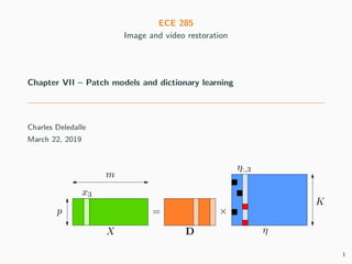
Instead of choosing the dictionary: wavelet basis, derivative filters, . . .
Can we learn it from a data-set x1, . . . , xm?
Sparsifying dictionary learning for images
Find a dictionary D = (d1, d2, . . . , dK ) ∈ Rn×K
, with K > n for redundancy,
such that the data-set X = (x1, x2, . . . , xm) ∈ Rn×m
can be represented by
sparse linear combinations of the atoms
D ∈ argmin
D∈Rn×K
min
η∈RK×m
1
2
m
j=1
||xj −
K
k=1
ηk,jdk||2
2
data fit
+ τ
m
j=1
K
k=1
|ηk,j|ρ
sparsity
= argmin
D∈Rn×K
min
η∈RK×m
1
2
||X − Dη||2
F
data fit
+ τ ||η||ρ
ρ
sparsity
.
Idea: find a dictionary that sparsifies the data-set.
9

D ∈ Rn×K
has too many degrees of freedom!
It cannot be estimated properly, and even then, it does not ﬁt in memory.
It would be feasible if the images were 8 × 8, but they are not.
10

Remarks: for wavelets and gradients, the atoms
1 have limited support 2 are stationary 3 are overlapping
D =




















d1 d2 . . . dK
d1 d2 . . . dK
d1 d2 . . . dK
...
d1 d2 . . . dK
d1 d2 . . . dK




















If we cannot learn D, can we learn the small atoms d1, . . . , dK ?
Ex: if the support is p = 8 × 8 and K = 512, the learning problem is tractable
even with a reasonable number K of training images xk.
11

Sparsifying dictionary learning for patches
Find a dictionary of patches D = (d1, d2, . . . , dK ) ∈ Rp×K
, with K > p for
redundancy, such that the data-set of patches X = (x1, x2, . . . , xm) ∈ Rp×m
can be represented by sparse linear combinations of the atoms
D ∈ argmin
D∈Rp×K
min
η∈RK×m
1
2
||X − Dη||2
F
data ﬁt
+ τ ||η||ρ,1
sparsity
.
12

D ∈ argmin
D∈Rp×K
min
η∈RK×m
1
2
||X − Dη||2
F
data ﬁt
+ τ ||η||ρ
ρ
sparsity
.
Optimization problem
• Add the constraint: ||dk||2 1,
Otherwise: D → ∞ and η → 0.
• For ρ 1:



• Convex with respect to D,
• Convex with respect to η,
• Non-convex with respect to (D, η).
• For ρ = 0:



• Convex with respect to D,
• Non-convex with respect to η,
• Non-convex with respect to (D, η).
13

Dictionary learning problem with k-SVD
D ∈ argmin
D∈Rp×K
min
η∈RK×m
1
2
||X − Dη||2
F
data fit
+ τ ||η||0
sparsity
subject to ||dk||2 1
k-SVD: Greedy algorithm for ρ = 0 (1/2) [Aharon et al., 2006]
1 Initialize D with normalized columns ||dk||2 = 1.
2 Sparse-coding stage: fix D and solve for each 1 j m
η:,j ∈ min
η∈RK
1
2
||xj − Dη||2
F
data fit
+ τ ||η||0
sparsity
with matching pursuit or orthogonal matching pursuit (see previous class).
14

Dictionary learning with k-SVD
k-SVD: Greedy algorithm for ρ = 0 (2/2) [Aharon et al., 2006]
3 Dictionary update: for all columns 1 k K
• Compute the residual without using the current atom dk:
Ek = X −
l=k
dlηl,: = X − (Dη − dkηk,:)
• ER
k : pick only the columns j of Ek for patches xj using atom dk,
• Update dk and ηk,: by ﬁnding the best rank 1 approximation
ER
k ≈ dkηk,: subject to ||dk||2 = 1
Use reduces SVD for rank 1 matrices:
ER
k = USV T
⇒ dk = U:,1 and ηk,: = S1,1V:,1
• Return to step 2 until convergence.
−→ k × SVD are performed at each iteration.
15

Update for atom k = 1
16

16

Update for atom k = K
16

A collection of 500 random patches (8x8) that were used for training, sorted
by their variance.
(a) (b) (c)
(a) The learned dictionary. Its elements are sorted in an ascending order of
their variance and stretched to maximal range for display purposes. (b) The
overcomplete separable Haar dictionary and (c) the over complete DCT
dictionary are used for comparison.
17

k-SVD based restoration (1/3) [Elad et al., 2006]
min
x∈Rn
η1,...,ηn∈RK
1
2σ2
||Hx − y||2
2
data ﬁt
+
n
i=1
β
2
||Pix − Dηi||2
2
patch approximation
+ τ||ηi||0
sparsity
(Half-Quadratic Splitting)
• x ∈ Rn
: unknown image,
• y = Hx + w ∈ Rq
: observed image with w ∼ N(0, σ2
Idq),
• H ∈ Rq×n
: blur, super-resolution, Radon transform. . .
• Pi ∈ Rp×n
: extract a patch of size p around pixel with index i,
• D ∈ Rp×K
: learned patch dictionary,
• ηi ∈ RK
: sparse code for patch with index i,
• β > 0, τ > 0: hyper-parameters.
Look for an image such that all its patches are well explained by sparse
linear combinations of learned atoms.
18

min
x∈Rn
η1,...,ηn∈RK
1
2σ2
||Hx − y||2
2
data ﬁt
+
n
i=1
β
2
||Pix − Dηi||2
2
patch approximation
+ τ||ηi||0
sparsity
Alternate minimization:
1 Initialize x, and repeat steps 2 and 3 until convergence,
2 Sparse coding: ﬁx x and solve for all index 1 i n
argmin
ηi∈RK
β
2
||Pix − Dηi||2
2
patch approximation
+ τ||ηi||0
sparsity
with matching pursuit or orthogonal matching pursuit (see previous class).
19

min
x∈Rn
η1,...,ηn∈RK
1
2σ2
||Hx − y||2
2
data fit
+
n
i=1
β
2
||Pix − Dηi||2
2
patch approximation
+ τ||ηi||0
sparsity
Alternate minimization:
3 Patch reprojection: for all ηi and solve for x
x ∈ argmin
x∈Rn
1
2σ2
||Hx − y||2
2
data fit
+
n
i=1
β
2
||Pix − Dηi||2
2
patch approximation
= H∗
H + σ2
β
n
i=1
P∗
i Pi
−1
H∗
y + σ2
β
n
i=1
P∗
i Dηi
• If H = Idn: average overlapping patches Dηi with the noisy image y
• Otherwise, solved by conjugate gradient, or efficiently depending on H.
20

Adaptively trained dictionary.
k-SVD for denoising
• Quality improvement: learned the dictionary on the noisy image itself,
• Speed-up: only once: sparse coding + reprojection (do not iterate).
21

k-SVD: Importance of redundancy Color k-SVD [Mairal et al., 2008]
Related works:
• Non-negative k-SVD [Aharon et al., 2005].
• Color k-SVD [Mairal et al., 2008].
• Analysis k-SVD [Rubinstein et al., 2013].
22

Sparsity with collaborative ﬁltering

Sparsity with collaborative ﬁltering
Motivations
• k-SVD:



• Patches are denoised independently,
• Use non-linear shrinkages to create sparsity,
• Use redundant learned dictionaries.
• Non-local Bayes:



• Denoise similar patches together,
• Use linear shrinkages (LMMSE),
• Use (non-local) orthogonal PCA basis.
Idea: use sparsity on stacks of similar patches.
23

Sparsity with collaborative ﬁltering – BM3D
BM3D: Block-matching and 3D ﬁltering [Dabov et al., 2007]
• Build groups of similar patches,
• Apply sparsifying 3D transform,
• Denoise each group (thresholding or LMMSE),
• Reproject/Aggregate overlapping patches.
Some results:
24

Grouping by matching
R is a targeting patch, other patches are grouped
with this patch by similarity (Euclidean distance).
25

Grouping by matching
Non-locality: patches that are far apart can be stacked together.
26

Grouping for collaborative filtering
• As groups contain similar patches:
• intrapatch correlation: peculiarity of natural images,
• interpatch correlation: results of grouping by similarity,
⇒ highly sparse representation.
R
Block matching
3D
grouping 3D transform Inverse 3D
transform
Denoised 3D
group
R R
-10 -5 0 5 10
-10
-8
-6
-4
-2
0
2
4
6
8
10
Filter / Shrinkage
Collaborative filtering:
• reveals finest details shared by similar patches,
• preserves unique features of each patch.
27

Aggregation
• Each pixel gets multiple estimates from diﬀerent groups
• Naive approach: average all estimates
. . . not all estimates are as good.
• Give higher weights to more reliable estimates
. . . measured according to their sparsity.
R
thr
thr
R
R R
Aggregation
28

Two steps filtering
• Noise may result in poor matching ⇒ degrades denoising performance.
• As for NL-Bayes, use two stages. At the second stage:
• Build stacks based on the similarity of pre-denoised patches,
• Use pre-denoised stacks to refine the shrinkage.
1 Step 1: Shrinkage: Hard thresholding with fixed threshold
3D trans.: Bi-orthogonal wavelets in space + Haar in 3rd dim.
2 Step 2: Shrinkage: LMMSE with signal variances deduced form step 1.
3D trans.: DCT in space + Haar in 3rd dim.
29

BM3D provides impressive results.
Since 2007, denoising results have not signiﬁcantly improved.
30

Adaptations to color and videos.
Color image denoising with BM3D [Dabov, 2007]
Video denoising with BM3D [Dabov, 2007]
31

Plug-and-play ADMM with BM3D
min
x∈Rn
E(x) =
1
2σ2
||y − Hx||2
2
F (x)
+R(x)
Adaptation to inverse-problems with Plug-and-play ADMM (1/2)
• Reminder: ADMM algorithm reads, for γ > 0, as
xk+1
= ProxγF (˜xk
+ dk
) (1)
˜xk+1
= ProxγR(xk+1
− dk
) (2)
dk+1
= dk
− xk+1
+ ˜xk+1
(1) ⇒ xk+1
= (σ2
Idn + γH∗
H)−1
(σ2
(˜xk
+ dk
) + γH∗
y) (inversion)
(2) ⇒ ˜xk+1
= argmin
z
1
2
||z − (xk+1
− dk
)||2
2 + γR(z) (denoising)
• Convergence when R is convex.
• Convergence when R is non-convex in some cases [Hong et al. 2016].
32

min
x∈Rn
E(x) =
1
2σ2
||y − Hx||2
2
F (x)
+R(x)
Adaptation to inverse-problems with Plug-and-play ADMM (2/2)
• Plug-and-play ADMM [Venkatakrishnan et al. 2013]
• Use any Gaussian denoiser for the denoising step
ex: (2) ⇒ ˜xk+1
= BM3D(xk+1
− dk
, γ)
• The regularization R is implicit.
• Convergence in some cases [Chan et al. 2016].
• Non-Gaussian noise: adapt F in (1) but (2) remains a Gaussian denoiser.
[Rond et al. 2015, Deledalle et al. 2017].
Simple solution allowing to use any of the many and very eﬃcient
Gaussian denoisers to solve diﬀerent kinds of image restoration problems.
33

ImagedomainWaveletdom.Fourierdom.
(a) Original image (b) Blurry image (c) Total-Variation (d) BM3D
Lost frequencies are recovered. Spatial contents and scales as well.
34

Sparsity and patch similarity – Denoising with NLSM
BM3D uses ﬁx dictionaries. Can we learn them `a la k-SVD?
Non-local sparse model (NLSM) [Mairal, 2009]
Learn a dictionary of patches:
• Use group sparsity for similar patches,
• Force similar patches to use the same
atoms (joint sparsity).
Then denoise each patch by sparse coding.
decomposition with joint sparsitysparse decomposition
non zero
coefficients
patches
patches
non zero
coefficients
patches
Some results:
35

Expected patch log-likelihood (EPLL)

Expected patch log-likelihood (1/2) [Zoran & Weiss, 2011]
• Use MAP with prior expressed on patches
min
x∈Rn
1
2σ2
||Hx − y||2
2
data ﬁt
+
n
i=1
− log p(Pix)
patch prior
• x ∈ Rn
: unknown image,
• y = Hx + w ∈ Rq
: observed image with w ∼ N(0, σ2
Idq),
• H ∈ Rq×n
: blur, super-resolution, Radon transform. . .
• Pi ∈ Rp×n
: extract a patch of size p around pixel with index i,
Look for an image such that all its patches are
well explained by the patch prior.
36

Expected patch log-likelihood (2/2) [Zoran & Weiss, 2011]
• Prior for a path zi = Pix ∈ Rp
, a Gaussian Mixture Model (GMM):
p(zi) =
K
k=1
wkN(zi; µk, Σk),
• wk > 0: weights of Gaussian component k ( k wk = 1),
• µk ∈ Rp
: mean of Gaussian component k,
• Σk ∈ Rp×p
: covariance matrix of Gaussian component k.
Represent the patch distribution by a superposition of ellipsoids.
37

Learning step
• Fit the distribution on a large dataset of clean patches:
input: x1, x2, . . . , xm clean patches
output: wk, µk, Σk for all 1 k K
• Standard choice:
• Dataset of m =2,000,000 patches,
• Patch size p = 8 × 8,
• Number of clusters K = 200.
• Use Expectation-Maximization algorithm [Dempster, 1977]
• Iterative algorithm similar to K-means,
• Greedy (maximizes the likelihood at each iteration),
• Converges to a local optimum (depending on the initialization).
38

Eigenvectors of 6 (among 200) covariance matrices of the learned GMM.
Some look like Fourier atoms while others model textures,
edges or other structures at diﬀerent scales and orientations.
39

min
x∈Rn
1
2σ2
||Hx − y||2
2 +
n
i=1
− log p(Pix)
Optimization by Half-Quadratic Splitting
• Use Half-Quadratic Splitting (as done in k-SVD)
min
x∈Rn
z1,...,zn∈Rp
1
2σ2
||Hx − y||2
2
data ﬁt
+
n
i=1
β
2
||Pix − zi||2
2
patch approximation
− log p(zi)
patch prior
with β > 0 an hyper-parameter.
• Alternate the minimization for all zi and x.
• Increase β after each iteration.
40

Greedy alternate minimization
• Repeat steps 1 and 2 (usually 5 iterations are enough):
1 Fix x and optimize for all patch zi:
min
zi∈Rp
β
2
||Pix − zi||2
2 +
n
i=1
− log
K
k=1
wkN(zi; µk, Σk)
• Prior is multi-modal: non-convex optimization problem.
• Look for the most likely Gaussian component ki given zi.
• Performs LMMSE with this Gaussian prior N(µki
, Σki
).
2 Fix zi and optimize for the image x:
min
x∈Rn
1
2σ2
||Hx − y||2
2 +
β
2
n
i=1
||Pix − zi||2
2
• Linear solution: same patch reprojection as for k-SVD (see slide 20).
41

Fast EPLL [Parameswaran et al., 2017]
1 Process only 3% of the patches at each iteration (chosen randomly),
2 Use a binary search tree to match for the best Gaussian component,
3 Approximate smallest eigenvalues of the covariance matrices.
⇒ 180× speed-up
(a) Random selection (b) Binary tree
10 20 30 40 50 60
10−3
10−1
95% 5%
Index of eigen dimension
Eigenvalue
data1
data2
data3
data4
(c) Cov. approx.
42

(a) Reference
22.1 / .368
(b) Noisy image
30.6 / .872 (1.68s)
(c) BM3D result
30.2 / .862 (0.36s)
(d) FEPLL result
Results of denoising (σ = 20)
43

(a) Reference / Blur kernel
24.9 / .624
(b) Blurry image
32.7 / .924 (0.46s)
(c) FEPLL result
Results of removing motion blur (subject to noise σ = 0.5)
44

Input
11.1 / .662 20.8 / .598 8.31 / .112
FEPLL
36.8 / .972 (0.38s)
(a) devignetting
23.3 / .738 (0.29s)
(b) ×3 super-resolution
27.0 / .905 (0.36s)
(c) 50% random inpainting
Various inverse problems (subject to noise σ = 2)
45

Other patch based restoration models

Patch based restoration models
Inpainting
Patch propagation [Xu and Sun, 2010]
• Inpaint progressively from the
edges of the missing region.
• Start with the pixels whose
patches are “rare” (i.e., sparse
similarity maps).
46

Super-resolution
Super-resolution from a single image [Glasner et al., 2009]
• Simulate multi-frames: use similar patches and their sub-pixel registration.
• Match patches from low-res and hi-res pairs.
magnification x3 (nearest neighbor, patch-based)
47

Deblurring
Adaptive sparse domain selection and regularization [Dong et al., 2011]
• Locally select dictionaries (sub-spaces),
• Perform sparse coding with the selected dictionary,
• Enforce stability under non-local ﬁltering.
blurry
total variation
minimization BM3D Dong 2009
patch based
48

What’s next?
Next open problems to deal with
• Blind denoising: statistics of the noise are unknown.
• Blind deconvolution: convolution kernel is unknown.
• Non-stationary blur: ex: moving objects, Bokeh. . .
• Non-linear degradations: ex: saturation, atmospheric turbulence. . .
(a) Motion blur (b) Bokeh (Mulholand drive, 2001) (c) Turbulence (OTIS dataset)
49

What’s next?
Next generations of restoration techniques
• Instead of learning statistics of images or patches, such as:
• Mean power spectral density (for Wiener ﬁltering),
• PCA (for LMMSE),
• Non-local PCA (for NL Bayes),
• Sparsifying dictionaries (k-SVD),
• Gaussian mixture models (EPLL).
⇒ Learn directly the algorithm.
What do all these algorithms have in common?
50

What’s next?
Non-Local means
for k in range(-s1, s1 + 1):
for l in range(-s2, s2 + 1):
yshift = shift(y, k, l) # Global linear
dist2 = (yshift - y)**2 # Pointwise non-linear
dist2 = convolve(dist2, nu) # Global linear
w = phi(dist2, sig, h, P * c) # Pointwise non-linear
x += w * yshift # Pointwise non-linear
Regularized anisotropic diﬀusion
for k in range(m-1):
gconv = grad(convolve(x, nu)) # Global linear
alpha = g(norm2(gconv)) # Pointwise non-linear
g = grad(z) # Global linear
v = alpha * g # Pointwise non-linear
x = x + gamma * div(v) # Global linear
ISTA+LASSO+UDWT+Deconvolution: BaB = WH∗
HW+
while condition:
z = z - gamma * (BaB(z) - Bay) # Global linear
z = SoftT(z, gamma * tau / lambda) # Pointwise non-linear
51

What’s next?
All restoration methods perform successions of:
• global linear operations (mixing everything):
ex: convolutions, shifts, patch extractions, aggregations, decimations...
• pointwise non-linear operations (taking decisions):
ex: thresholdings, exponentials, squares, element-wise products...
These are artiﬁcial (deep convolutional) Neural Networks (NNs).
Instead of designing all steps yourself, let the machine learn them.
52

What’s next?
Fast Super-Resolution Convolutional NN [Dong et al., 2016]
BM3D-Net [Yang & Sun, 2017]
Want to learn more?
Fall quarter 2019: Machine Learning for Image Processing
53

Questions?
That’s all folks!
Sources and images courtesy of
• L. Denis
• J. Gilles
• G. Peyr´e
• W. Sharba
• F. Tupin
• Wikipedia
53

IVR - Chapter 7 - Patch models and dictionary learning

Recommended

Recommended

More Related Content

What's hot

What's hot (20)

Similar to IVR - Chapter 7 - Patch models and dictionary learning

Similar to IVR - Chapter 7 - Patch models and dictionary learning (20)

More from Charles Deledalle

More from Charles Deledalle (11)

Recently uploaded

Recently uploaded (20)

IVR - Chapter 7 - Patch models and dictionary learning