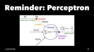
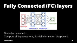
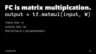
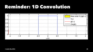
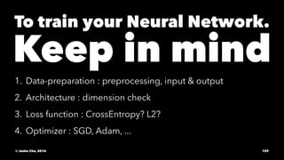
Download as PDF, PPTX


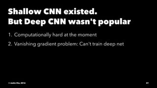
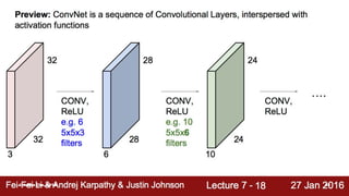
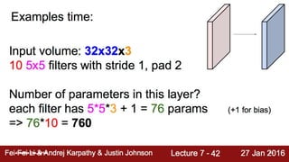
![This is Typical Convolutional
Neural Network (CNN)
[LeNet-5, LeCun 1980]
© Junho Cho, 2016 18](https://image.slidesharecdn.com/cnn-170610061501/85/Convolutional-Neural-Network-18-320.jpg)
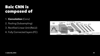
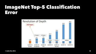
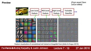
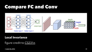
![Basic CNN
[(Conv-ReLU)*n - POOL] * m - (FC-ReLU) * k - loss
that's it! for real
© Junho Cho, 2016 20](https://image.slidesharecdn.com/cnn-170610061501/85/Convolutional-Neural-Network-20-320.jpg)


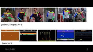
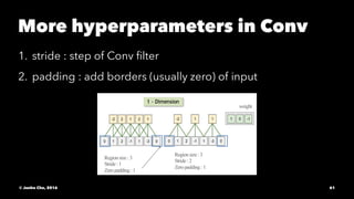
![[LeNet-5, LeCun 1980]
© Junho Cho, 2016 26](https://image.slidesharecdn.com/cnn-170610061501/85/Convolutional-Neural-Network-26-320.jpg)


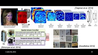


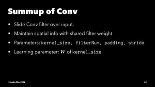

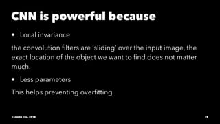


![How they look in code?
def model(X, w, w2, w3, w4, w_o, p_keep_conv, p_keep_hidden):
l1a = tf.nn.relu(tf.nn.conv2d(X, w,
strides=[1, 1, 1, 1], padding='SAME'))
# l1a output shape=(?, input_height, input_width, number_of_channels_layer1)
l1 = tf.nn.max_pool(l1a, ksize=[1, 2, 2, 1],
strides=[1, 2, 2, 1], padding='SAME')
# l1 output shape=(?, input_height/2, input_width/2, number_of_channels_layer1)
l1 = tf.nn.dropout(l1, p_keep_conv)
l2a = tf.nn.relu(tf.nn.conv2d(l1, w2,
strides=[1, 1, 1, 1], padding='SAME'))
# l2a output shape=(?, input_height/2, input_width/2, number_of_channels_layer2)
l2 = tf.nn.max_pool(l2a, ksize=[1, 2, 2, 1],
strides=[1, 2, 2, 1], padding='SAME')
# l2 shape=(?, input_height/4, input_width/4, number_of_channels_layer2)
l2 = tf.nn.dropout(l2, p_keep_conv)
l3a = tf.nn.relu(tf.nn.conv2d(l2, w3,
strides=[1, 1, 1, 1], padding='SAME'))
# l3a shape=(?, input_height/4, input_width/4, number_of_channels_layer3)
l3 = tf.nn.max_pool(l3a, ksize=[1, 2, 2, 1],
strides=[1, 2, 2, 1], padding='SAME')
# l3 shape=(?, input_height/8, input_width/8, number_of_channels_layer3)
l3 = tf.reshape(l3, [-1, w4.get_shape().as_list()[0]])
# flatten to (?, input_height/8 * input_width/8 * number_of_channels_layer3)
l3 = tf.nn.dropout(l3, p_keep_conv)
l4 = tf.nn.relu(tf.matmul(l3, w4))
#fully connected_layer
l4 = tf.nn.dropout(l4, p_keep_hidden)
pyx = tf.matmul(l4, w_o)
return pyx
© Junho Cho, 2016 91](https://image.slidesharecdn.com/cnn-170610061501/85/Convolutional-Neural-Network-91-320.jpg)


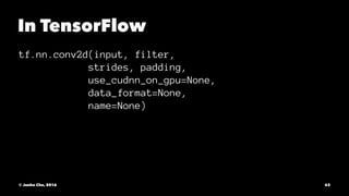
![Define model
def model(X, w, w2, w3, w4, w_o, p_keep_conv, p_keep_hidden):
l1a = tf.nn.relu(tf.nn.conv2d(X, w,
strides=[1, 1, 1, 1], padding='SAME'))
# l1a output shape=(?, input_height, input_width, number_of_channels_layer1)
l1 = tf.nn.max_pool(l1a, ksize=[1, 2, 2, 1],
strides=[1, 2, 2, 1], padding='SAME')
# l1 output shape=(?, input_height/2, input_width/2, number_of_channels_layer1)
l1 = tf.nn.dropout(l1, p_keep_conv)
l2a = tf.nn.relu(tf.nn.conv2d(l1, w2,
strides=[1, 1, 1, 1], padding='SAME'))
# l2a output shape=(?, input_height/2, input_width/2, number_of_channels_layer2)
l2 = tf.nn.max_pool(l2a, ksize=[1, 2, 2, 1],
strides=[1, 2, 2, 1], padding='SAME')
# l2 shape=(?, input_height/4, input_width/4, number_of_channels_layer2)
l2 = tf.nn.dropout(l2, p_keep_conv)
l3a = tf.nn.relu(tf.nn.conv2d(l2, w3,
strides=[1, 1, 1, 1], padding='SAME'))
# l3a shape=(?, input_height/4, input_width/4, number_of_channels_layer3)
l3 = tf.nn.max_pool(l3a, ksize=[1, 2, 2, 1],
strides=[1, 2, 2, 1], padding='SAME')
# l3 shape=(?, input_height/8, input_width/8, number_of_channels_layer3)
l3 = tf.reshape(l3, [-1, w4.get_shape().as_list()[0]])
# flatten to (?, input_height/8 * input_width/8 * number_of_channels_layer3)
l3 = tf.nn.dropout(l3, p_keep_conv)
l4 = tf.nn.relu(tf.matmul(l3, w4))
#fully connected_layer
l4 = tf.nn.dropout(l4, p_keep_hidden)
pyx = tf.matmul(l4, w_o)
return pyx
© Junho Cho, 2016 118](https://image.slidesharecdn.com/cnn-170610061501/85/Convolutional-Neural-Network-118-320.jpg)

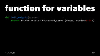
![Initialize
w = init_weights([3, 3, 1, 32])
w2 = init_weights([3, 3, 32, 64])
w3 = init_weights([3, 3, 64, 128])
w4 = init_weights([128 * 4 * 4, 625])
w_o = init_weights([625, 10])
p_keep_conv = tf.placeholder(tf.float32)
p_keep_hidden = tf.placeholder(tf.float32)
py_x = model(X, w, w2, w3, w4, w_o, p_keep_conv, p_keep_hidden)
© Junho Cho, 2016 120](https://image.slidesharecdn.com/cnn-170610061501/85/Convolutional-Neural-Network-120-320.jpg)
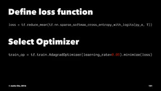

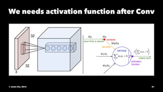
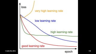
![Monitor accuracy of my model
correct = tf.nn.in_top_k(py_x, Y, 1)
accuracy = tf.reduce_mean(tf.cast(correct, tf.float32))
Monitor my loss function drop
x = np.arange(50)
plt.plot(x, trn_loss_list)
plt.plot(x, test_loss_list)
plt.title("cross entropy loss")
plt.legend(["train loss", "test_loss"])
plt.xlabel("epoch")
plt.ylabel("cross entropy")
© Junho Cho, 2016 123](https://image.slidesharecdn.com/cnn-170610061501/85/Convolutional-Neural-Network-123-320.jpg)


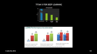


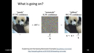


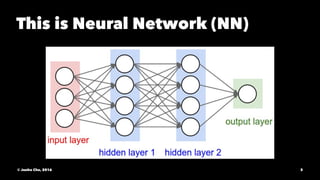
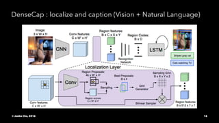
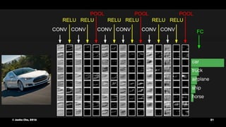
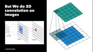
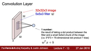
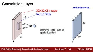
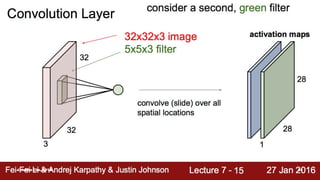
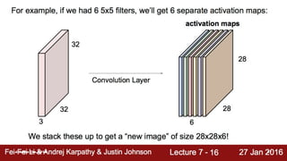
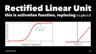
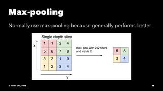
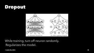
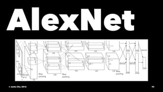
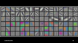
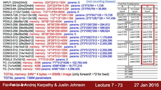
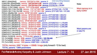
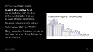
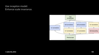
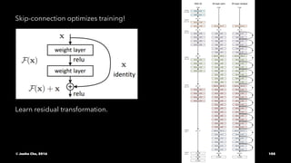
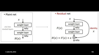
The document provides an overview of convolutional neural networks (CNNs) presented by Junho Cho. It discusses the basic components of CNNs including convolution, pooling, rectified linear units (ReLU), and fully connected layers. It also reviews popular CNN architectures such as LeNet, AlexNet, VGGNet, GoogLeNet, and ResNet. The document emphasizes that CNNs are powerful due to their ability to learn local invariance through the use of convolutional filters and sharing weights, while also having fewer parameters than fully connected networks to prevent overfitting. Finally, it provides code examples for implementing CNN models in TensorFlow.


![7.__Developing_a_Research_Proposal[1].pptx](https://cdn.slidesharecdn.com/ss_thumbnails/7-260131073037-df92dd7d-thumbnail.jpg?width=640&height=640&fit=bounds)


