Principal component analysis is a useful multivariate times series method to examine and study the drivers of the changes in the entire dataset. The main advantage of PCA is the reduction of dimensionality where the large sets of data get transformed into few principal factors that explain majority of variability in that group. PCA has found many applications in finance – both in risk and yield curve analytics

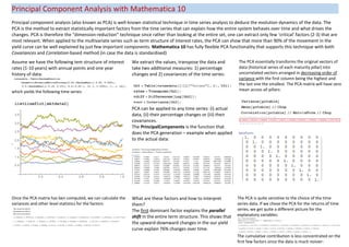
1. Principal Component Analysis with Mathematica 10
Principal component analysis (also known as PCA) is well-known statistical technique in time series analysis to deduce the evolution dynamics of the data. The PCA is the method to extract statistically important factors from the time series that can explain how the entire system behaves over time and what drives the changes. PCA is therefore the “dimension-reduction” technique since rather than looking at the entire set, one can extract only few ‘critical’ factors (2-3) that are most relevant. When applied to the multivariate series such as term structure of interest rates, the PCA can show that more than 90% of the movement in the yield curve can be well explained by just few important components. Mathematica 10 has fully flexible PCA functionality that supports this technique with both Covariances and Correlation-based method (in case the data is standardised)
Assume we have the following tem structure of interest rates (1-10 years) with annual points and one year history of data:
which yields the following time series:
We extract the values, transpose the data and take two additional measures: 1) percentage changes and 2) covariances of the time series:
PCA can be applied to any time series: (i) actual data, (ii) their percentage changes or (iii) their covariances.
The PrincipalCompenents is the function that does the PCA generation – example when applied to the actual data:
The PCA essentially transforms the original vectors of data (historical series of each maturity pillar) into uncorrelated vectors arranged in decreasing order of variance with the first column being the highest and the last one the smallest. The PCA matrix will have zero mean across all pillars:
Once the PCA matrix has ben computed, we can calculate the variances and other level statistics for the factors:
What are these factors and how to interpret them?
The first dominant factor explains the parallel shift in the entire term structure. This shows that the upward-downward changes in the our yield curve explain 76% changes over time.
The PCA is quite sensitive to the choice of the time series data. If we chose the PCA for the returns of time series, we get quite a different picture for the explanatory variables:
The cumulative contribution is less concentrated on the first few factors since the data is much noisier:

2. It is of a particular interest to look at the cumulative weight of the variance over the entire columns set:
As we can see, the first 3 factors explain 92% variation of the entire tem structure:
The second component explains the slope of the curve, or the rotation of the yield curve. The second factor explains 11% of the changes and the first two combined produce 87% explanation of the rates changes.
The third factor explains the curvature in the term structure, or its convexity. Its contribution to the explanatory scheme stands at 5% and all three factors together make 92% explanation of all changes in the time series.
We can decompose each factor par pillar. This is the parallel shift:
With his setting, the curvature impact on the term structure will look as follows: