1 linear algebra matrices

256
C H A P T E R 7
Linear Algebra: Matrices,
Vectors, Determinants.
Linear Systems
Linear algebra is a fairly extensive subject that covers vectors and matrices, determinants,
systems of linear equations, vector spaces and linear transformations, eigenvalue problems,
and other topics. As an area of study it has a broad appeal in that it has many applications
in engineering, physics, geometry, computer science, economics, and other areas. It also
contributes to a deeper understanding of mathematics itself.
Matrices, which are rectangular arrays of numbers or functions, and vectors are the
main tools of linear algebra. Matrices are important because they let us express large
amounts of data and functions in an organized and concise form. Furthermore, since
matrices are single objects, we denote them by single letters and calculate with them
directly. All these features have made matrices and vectors very popular for expressing
scientific and mathematical ideas.
The chapter keeps a good mix between applications (electric networks, Markov
processes, traffic flow, etc.) and theory. Chapter 7 is structured as follows: Sections 7.1
and 7.2 provide an intuitive introduction to matrices and vectors and their operations,
including matrix multiplication. The next block of sections, that is, Secs. 7.3–7.5 provide
the most important method for solving systems of linear eq uations by the Gauss
elimination method. This method is a cornerstone of linear algebra, and the method
itself and variants of it appear in different areas of mathematics and in many applications.
It leads to a consideration of the behavior of solutions and concepts such as rank of a
matrix, linear independence, and bases. We shift to determinants, a topic that has
declined in importance, in Secs. 7.6 and 7.7. Section 7.8 covers inverses of matrices.
The chapter ends with vector spaces, inner product spaces, linear transformations, and
composition of linear transformations. Eigenvalue problems follow in Chap. 8.
COMMENT. N umeric linear algeb ra ( Secs. 2 0 .1 – 2 0 .5 ) can b e studied immediately
after this chapter.
Prerequisite: None.
Sections that may be omitted in a short course: 7.5, 7.9.
R eferences and Answers to Problems: App. 1 Part B, and App. 2.
c 07.qxd 10/28/10 7:30 PM Page 256

7.1 Matrices, Vectors:
Addition and Scalar Multiplication
The basic concepts and rules of matrix and vector algebra are introduced in Secs. 7.1 and
7.2 and are followed by linear systems (systems of linear equations), a main application,
in Sec. 7.3.
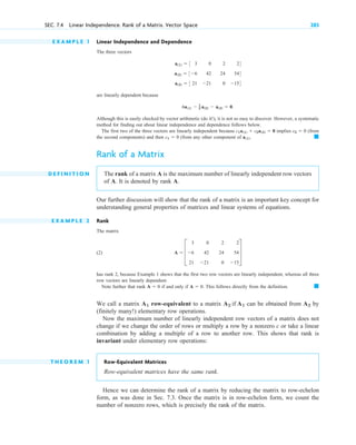
Let us first take a leisurely look at matrices before we formalize our discussion. A matrix
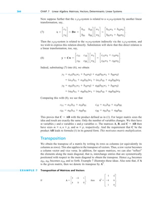
is a rectangular array of numbers or functions which we will enclose in brackets. For example,
(1)
are matrices. The numbers (or functions) are called entries or, less commonly, elements
of the matrix. The first matrix in (1) has two rows, which are the horizontal lines of entries.
Furthermore, it has three columns, which are the vertical lines of entries. The second and
third matrices are square matrices, which means that each has as many rows as columns—
3 and 2, respectively. The entries of the second matrix have two indices, signifying their
location within the matrix. The first index is the number of the row and the second is the
number of the column, so that together the entry’s position is uniquely identified. For
example, (read a two three) is in Row 2 and Column 3, etc. The notation is standard
and applies to all matrices, including those that are not square.
Matrices having just a single row or column are called vectors. Thus, the fourth matrix
in (1) has just one row and is called a row vector. The last matrix in (1) has just one
column and is called a column vector. Because the goal of the indexing of entries was
to uniquely identify the position of an element within a matrix, one index suffices for
vectors, whether they are row or column vectors. Thus, the third entry of the row vector
in (1) is denoted by
Matrices are handy for storing and processing data in applications. Consider the
following two common examples.
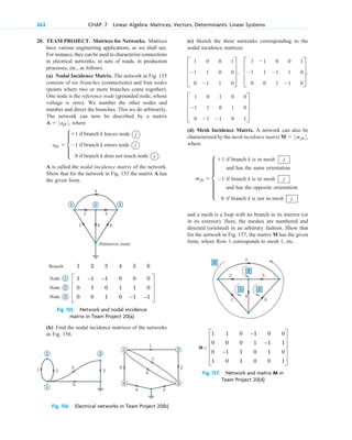
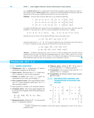
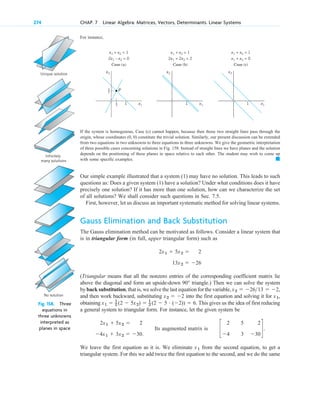
E X A M P L E 1 Linear Systems, a Major Application of Matrices
We are given a system of linear equations, briefly a linear system, such as
where are the unknowns. We form the coefficient matrix, call it A, by listing the coefficients of the
unknowns in the position in which they appear in the linear equations. In the second equation, there is no
unknown which means that the coefficient of is 0 and hence in matrix A, Thus,
a22 0,
x2
x2,
x1, x2, x3
4x1 6x2 9x3 6
6x1 2x3 20
5x1 8x2 x3 10
a3.
a23
c
eⴚx
2x2
e6x
4x
d, [ a1 a2 a3] , c
4
1
2
d
c
0.3 1 5
0 0.2 16
d, D
a11 a12 a13
a21 a22 a23
a31 a32 a33
T,
SEC. 7.1 Matrices, Vectors: Addition and Scalar Multiplication 257
c 07.qxd 10/28/10 7:30 PM Page 257

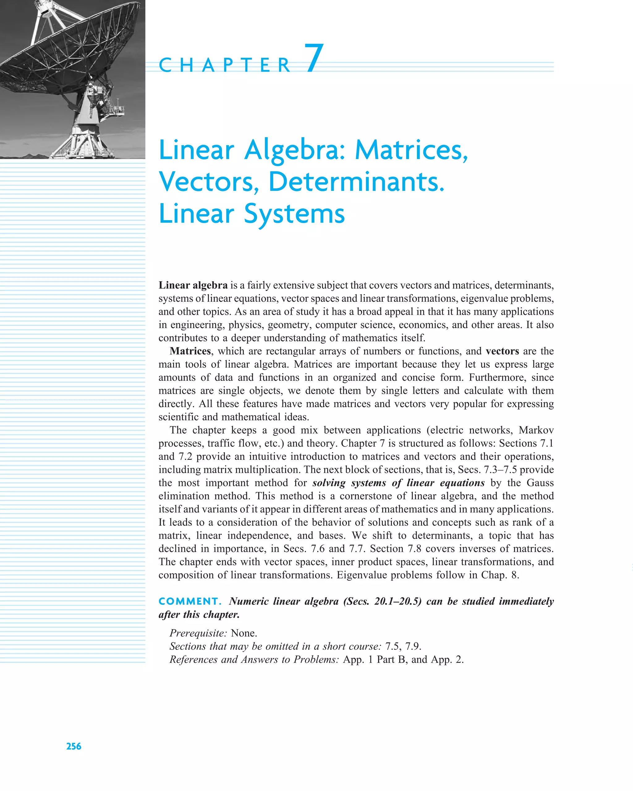
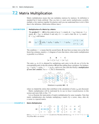
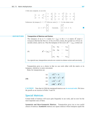
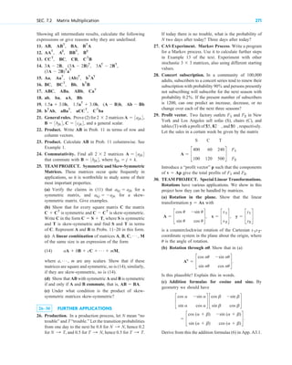
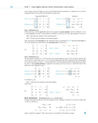
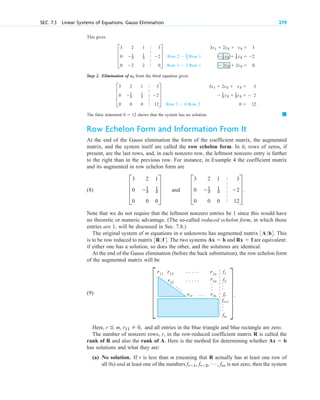
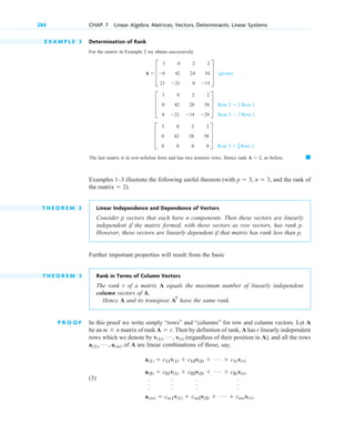
by augmenting A with the right sides of the linear system and call it the augmented matrix of the system.
Since we can go back and recapture the system of linear equations directly from the augmented matrix ,
contains all the information of the system and can thus be used to solve the linear system. This means that we
can just use the augmented matrix to do the calculations needed to solve the system. We shall explain this in
detail in Sec. 7.3. Meanwhile you may verify by substitution that the solution is .
The notation for the unknowns is practical but not essential; we could choose x, y, z or some other
letters.
E X A M P L E 2 Sales Figures in Matrix Form
Sales figures for three products I, II, III in a store on Monday (Mon), Tuesday (Tues), may for each week
be arranged in a matrix
If the company has 10 stores, we can set up 10 such matrices, one for each store. Then, by adding corresponding
entries of these matrices, we can get a matrix showing the total sales of each product on each day. Can you think
of other data which can be stored in matrix form? For instance, in transportation or storage problems? Or in
listing distances in a network of roads?
General Concepts and Notations
Let us formalize what we just have discussed. We shall denote matrices by capital boldface
letters A, B, C, , or by writing the general entry in brackets; thus , and so
on. By an matrix (read m by n matrix) we mean a matrix with m rows and n
columns— rows always come first! is called the size of the matrix. Thus an
matrix is of the form
(2)
The matrices in (1) are of sizes and respectively.
Each entry in (2) has two subscripts. The first is the row number and the second is the
column number. Thus is the entry in Row 2 and Column 1.
If we call A an square matrix. Then its diagonal containing the entries
is called the main diagonal of A. Thus the main diagonals of the two
square matrices in (1) are and respectively.
Square matrices are particularly important, as we shall see. A matrix of any size
is called a rectangular matrix; this includes square matrices as a special case.
m n
eⴚx
, 4x,
a11, a22, a33
a11, a22, Á , ann
n n
m n,
a21
2 1,
2 3, 3 3, 2 2, 1 3,
A 3ajk4 E
a11 a12
Á a1n
a21 a22
Á a2n
# # Á #
am1 am2
Á amn
U .
m n
m n
m ⴛ n
A [ ajk]
Á
䊏
A
Mon Tues Wed Thur Fri Sat Sun
40 33 81 0 21 47 33
D 0 12 78 50 50 96 90 T
10 0 0 27 43 78 56
#
I
II
III
Á
䊏
x1, x2, x3
x1 3, x2 1
2, x3 1
A
~
A
~
A D
4 6 9
6 0 2
5 8 1
T. We form another matrix A
~
D
4 6 9 6
6 0 2 20
5 8 1 10
T
258 CHAP. 7 Linear Algebra: Matrices, Vectors, Determinants. Linear Systems
c 07.qxd 10/28/10 7:30 PM Page 258

Vectors
A vector is a matrix with only one row or column. Its entries are called the components
of the vector. We shall denote vectors by lowercase boldface letters a, b, or by its
general component in brackets, , and so on. Our special vectors in (1) suggest
that a (general) row vector is of the form
A column vector is of the form
Addition and Scalar Multiplication
of Matrices and Vectors
What makes matrices and vectors really useful and particularly suitable for computers is
the fact that we can calculate with them almost as easily as with numbers. Indeed, we
now introduce rules for addition and for scalar multiplication (multiplication by numbers)
that were suggested by practical applications. (Multiplication of matrices by matrices
follows in the next section.) We first need the concept of equality.
D E F I N I T I O N Equality of Matrices
Two matrices and are equal, written if and only if
they have the same size and the corresponding entries are equal, that is,
and so on. Matrices that are not equal are called different. Thus, matrices
of different sizes are always different.
E X A M P L E 3 Equality of Matrices
Let
Then
The following matrices are all different. Explain!
䊏
c
1 3
4 2
d c
4 2
1 3
d c
4 1
2 3
d c
1 3 0
4 2 0
d c
0 1 3
0 4 2
d
A B if and only if
a11 4, a12 0,
a21 3, a22 1.
A c
a11 a12
a21 a22
d and B c
4 0
3 1
d.
a12 b12,
a11 b11,
A B,
B 3bjk4
A 3ajk4
b E
b1
b2
.
.
.
bm
U . For instance, b D
4
0
7
T.
a 3a1 a2
Á an4. For instance, a 32 5 0.8 0 14.
a 3aj4
Á
c 07.qxd 10/28/10 7:30 PM Page 259

D E F I N I T I O N Addition of Matrices
The sum of two matrices and of the same size is written
and has the entries obtained by adding the corresponding entries
of A and B. Matrices of different sizes cannot be added.
As a special case, the sum of two row vectors or two column vectors, which
must have the same number of components, is obtained by adding the corresponding
components.
E X A M P L E 4 Addition of Matrices and Vectors
If and , then .
A in Example 3 and our present A cannot be added. If and , then
.
An application of matrix addition was suggested in Example 2. Many others will follow.
D E F I N I T I O N Scalar Multiplication (Multiplication by a Number)
The product of any matrix and any scalar c (number c) is written
cA and is the matrix obtained by multiplying each entry of A
by c.
Here is simply written and is called the negative of A. Similarly, is
written . Also, is written and is called the difference of A and B
(which must have the same size! ).
E X A M P L E 5 Scalar Multiplication
If , then
If a matrix B shows the distances between some cities in miles, 1.609B gives these distances in kilometers.
Rules for Matrix Addition and Scalar Multiplication. From the familiar laws for the
addition of numbers we obtain similar laws for the addition of matrices of the same size
, namely,
(a)
(3)
(b) (written )
(c)
(d) .
Here 0 denotes the zero matrix (of size ), that is, the matrix with all entries
zero. If or , this is a vector, called a zero vector.
n 1
m 1
m n
m n
A (A) 0
A 0 A
A B C
(A B) C A (B C)
A B B A
m n
䊏
A D
2.7 1.8
0 0.9
9.0 4.5
T,
10
9
A D
3
0
10
2
1
5
T, 0A D
0
0
0
0
0
0
T.
A D
2.7
0
9.0
1.8
0.9
4.5
T
A B
A (B)
kA
(k)A
A
(1)A
cA 3cajk4
m n
A 3ajk4
m n
䊏
a b 31 9 24
b 36 2 04
a 35 7 24
A B c
1 5 3
3 2 2
d
B c
5 1 0
3 1 0
d
A c
4 6 3
0 1 2
d
a b
ajk bjk
A B
B 3bjk4
A 3ajk4
c 07.qxd 10/28/10 7:30 PM Page 260

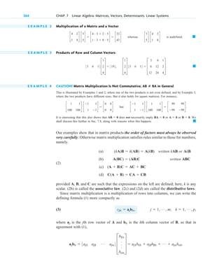
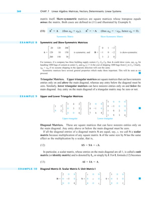
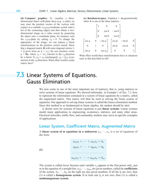
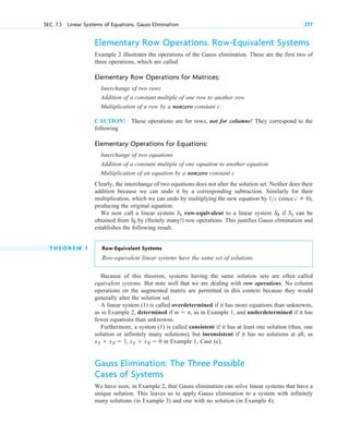
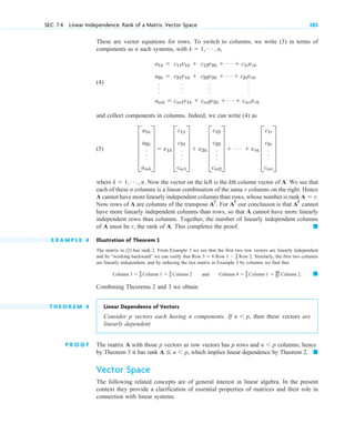
1–7 GENERAL QUESTIONS
1. Equality. Give reasons why the five matrices in
Example 3 are all different.
2. Double subscript notation. If you write the matrix in
Example 2 in the form , what is
? ?
3. Sizes. What sizes do the matrices in Examples 1, 2, 3,
and 5 have?
4. Main diagonal. What is the main diagonal of A in
Example 1? Of A and B in Example 3?
5. Scalar multiplication. If A in Example 2 shows the
number of items sold, what is the matrix B of units sold
if a unit consists of (a) 5 items and (b) 10 items?
6. If a matrix A shows the distances between
12 cities in kilometers, how can you obtain from A the
matrix B showing these distances in miles?
7. Addition of vectors. Can you add: A row and
a column vector with different numbers of compo-
nents? With the same number of components? Two
row vectors with the same number of components
but different numbers of zeros? A vector and a
scalar? A vector with four components and a
matrix?
8–16 ADDITION AND SCALAR
MULTIPLICATION OF MATRICES
AND VECTORS
Let
C D
5
2
1
2
4
0
T, D D
4
5
2
1
0
1
T,
A D
0
6
1
2
5
0
4
5
3
T, B D
0
5
2
5
3
4
2
4
2
T
2 2
12 12
a33
a26
a13?
a31?
A 3ajk4
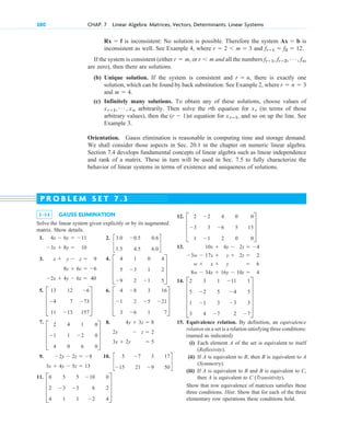
P R O B L E M S E T 7 . 1
Find the following expressions, indicating which of the
rules in (3) or (4) they illustrate, or give reasons why they
are not defined.
8.
9.
10.
11.
12.
13.
14.
15.
16.
17. Resultant of forces. If the above vectors u, v, w
represent forces in space, their sum is called their
resultant. Calculate it.
18. Equilibrium. By definition, forces are in equilibrium
if their resultant is the zero vector. Find a force p such
that the above u, v, w, and p are in equilibrium.
19. General rules. Prove (3) and (4) for general
matrices and scalars c and k.
2 3
8.5w 11.1u 0.4v
15v 3w 0u, 3w 15v, D u 3C,
0E u v
(u v) w, u (v w), C 0w,
10(u v) w
E (u v),
(5u 5v) 1
2 w, 20(u v) 2w,
(2 # 7)C, 2(7C), D 0E, E D C u
A 0C
(C D) E, (D E) C, 0(C E) 4D,
0.6(C D)
8C 10D, 2(5D 4C), 0.6C 0.6D,
(4 # 3)A, 4(3A), 14B 3B, 11B
3A, 0.5B, 3A 0.5B, 3A 0.5B C
2A 4B, 4B 2A, 0A B, 0.4B 4.2A
u D
1.5
0
3.0
T, v D
1
3
2
T, w D
5
30
10
T.
E D
0
3
3
2
4
1
T
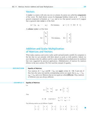
Hence matrix addition is commutative and associative [ by (3a) and (3b)] .
Similarly, for scalar multiplication we obtain the rules
(a)
(4)
(b)
(c) (written ckA)
(d) 1A A.
c(kA) (ck)A
(c k)A cA kA
c(A B) cA cB
c 07.qxd 10/28/10 7:30 PM Page 261

20. TEAM PROJECT. Matrices for Networks. Matrices
have various engineering applications, as we shall see.
For instance, they can be used to characterize connections
in electrical networks, in nets of roads, in production
processes, etc., as follows.
(a) Nodal Incidence Matrix. The network in Fig. 155
consists of six branches (connections) and four nodes
(points where two or more branches come together).
One node is the reference node (grounded node, whose
voltage is zero). We number the other nodes and
number and direct the branches. This we do arbitrarily.
The network can now be described by a matrix
, where
A is called the nodal incidence matrix of the network.
Show that for the network in Fig. 155 the matrix A has
the given form.
ajk d
1 if branch k leaves node j
1 if branch k enters node j
0 if branch k does not touch node j .
A 3ajk4
(c) Sketch the three networks corresponding to the
nodal incidence matrices
(d) Mesh Incidence Matrix. A network can also be
characterized by the mesh incidence matrix
where
and a mesh is a loop with no branch in its interior (or
in its exterior). Here, the meshes are numbered and
directed (oriented) in an arbitrary fashion. Show that
for the network in Fig. 157, the matrix M has the given
form, where Row 1 corresponds to mesh 1, etc.
1 if branch k is in mesh j
and has the same orientation
1 if branch k is in mesh j
and has the opposite orientation
0 if branch k is not in mesh j
mjk f
M 3mjk4,
D
1 0 1 0 0
1 1 0 1 0
0 1 1 0 1
T.
D
1 1 0 0 1
1 1 1 1 0
0 0 1 1 0
T,
D
1 0 0 1
1 1 0 0
0 1 1 0
T,
1 6
1 2
3
4
2 5
3
4
1 1
0
–1
0
0
0 –1
1
0
0
1
0 0
1
0
–1
1
0
1 0
1 1
0
M =
1 6
1
2 5
4
3
2 3
(Reference node)
Branch 1
1
2
–1
1
0
3 4 5
Node 1
0
Node 2
0
–1 0
1
0
0
1
0
1
–1
Node 3
6
0
0
–1
Fig. 155. Network and nodal incidence
matrix in Team Project 20(a)
1
2 3
4
5
3
2
1
2
5
3
4
1
7
6
1 2
3
4
Fig. 156. Electrical networks in Team Project 20(b)
Fig. 157. Network and matrix M in
Team Project 20(d)
(b) Find the nodal incidence matrices of the networks
in Fig. 156.
c 07.qxd 10/28/10 7:30 PM Page 262

where we shaded the entries that contribute to the calculation of entry just discussed.
Matrix multiplication will be motivated by its use in linear transformations in this
section and more fully in Sec. 7.9.
Let us illustrate the main points of matrix multiplication by some examples. Note that
matrix multiplication also includes multiplying a matrix by a vector, since, after all,
a vector is a special matrix.
E X A M P L E 1 Matrix Multiplication
Here and so on. The entry in the box is
The product BA is not defined. 䊏
c23 4 # 3 0 # 7 2 # 1 14.
c11 3 # 2 5 # 5 (1) # 9 22,
AB D
3
4
6
5
0
3
1
2
2
T D
2
5
9
2
0
4
3
7
1
1
8
1
T D
22
26
9
2
16
4
43
14
37
42
6
28
T
c21
SEC. 7.2 Matrix Multiplication 263
7.2 Matrix Multiplication
Matrix multiplication means that one multiplies matrices by matrices. Its definition is
standard but it looks artificial. Thus you have to study matrix multiplication carefully,
multiply a few matrices together for practice until you can understand how to do it. Here
then is the definition. (Motivation follows later.)
D E F I N I T I O N Multiplication of a Matrix by a Matrix
The product (in this order) of an matrix times an
matrix is defined if and only if and is then the matrix
with entries
(1)
The condition means that the second factor, B, must have as many rows as the first
factor has columns, namely n. A diagram of sizes that shows when matrix multiplication
is possible is as follows:
The entry in (1) is obtained by multiplying each entry in the jth row of A by the
corresponding entry in the kth column of B and then adding these n products. For instance,
and so on. One calls this briefly a multiplication
of rows into columns. For , this is illustrated by
n 3
c21 a21b11 a22b21 Á a2nbn1,
cjk
A B C
3m n4 3n p4 3m p4.
r n
cjk a
n
l1
ajlblk aj1b1k aj2b2k Á ajnbnk
j 1, Á , m
k 1, Á , p.
C 3cjk4
m p
r n
B 3bjk4
r p
A 3ajk4
m n
C AB
a11
a12
a13
a21
a22
a23
a31
a32
a33
a41
a42
a43
m = 4
m = 4
n = 3
=
c11
c12
c21
c22
c31
c32
c41
c42
b11
b12
b21
b22
b31
b32
p = 2 p = 2
Notations in a product AB C
c 07.qxd 10/28/10 7:30 PM Page 263

E X A M P L E 2 Multiplication of a Matrix and a Vector
whereas is undefined.
E X A M P L E 3 Products of Row and Column Vectors
E X A M P L E 4 CAUTION! Matrix Multiplication Is Not Commutative, in General
This is illustrated by Examples 1 and 2, where one of the two products is not even defined, and by Example 3,
where the two products have different sizes. But it also holds for square matrices. For instance,
but
It is interesting that this also shows that does not necessarily imply or or . We
shall discuss this further in Sec. 7.8, along with reasons when this happens.
Our examples show that in matrix products the order of factors must always b e ob served
very carefully. Otherwise matrix multiplication satisfies rules similar to those for numbers,
namely.
(a) written kAB or AkB
(2)
(b) written ABC
(c)
(d)
provided A, B, and C are such that the expressions on the left are defined; here, k is any
scalar. (2b) is called the associative law. (2c) and (2d) are called the distributive laws.
Since matrix multiplication is a multiplication of rows into columns, we can write the
defining formula (1) more compactly as
(3)
where is the jth row vector of A and is the kth column vector of B, so that in
agreement with (1),
ajbk 3aj1 aj2
Á ajn4 D
b1k
.
.
.
bnk
T aj1b1k aj2b2k Á ajnbnk.
bk
aj
j 1, Á , m; k 1, Á , p,
cjk ajbk,
C(A B) CA CB
(A B)C AC BC
A(BC) (AB)C
(kA)B k(AB) A(kB)
䊏
B 0
A 0
BA 0
AB 0
c
1
1
1
1
d c
1
100
1
100
d c
99
99
99
99
d.
c
1
100
1
100
d c
1
1
1
1
d c
0
0
0
0
d
AB ⴝ BA
䊏
D
1
2
4
T 33 6 14 D
3
6
12
6
12
24
1
2
4
T.
33 6 14 D
1
2
4
T 3194,
䊏
c
3
5
d c
4
1
2
8
d
c
4
1
2
8
d c
3
5
d c
4 # 3 2 # 5
1 # 3 8 # 5
d c
22
43
d
c 07.qxd 10/28/10 7:30 PM Page 264

E X A M P L E 5 Product in Terms of Row and Column Vectors
If is of size and is of size then
(4)
Taking etc., verify (4) for the product in Example 1.
Parallel processing of products on the computer is facilitated by a variant of (3) for
computing , which is used by standard algorithms (such as in Lapack). In this
method, A is used as given, B is taken in terms of its column vectors, and the product is
computed columnwise; thus,
(5)
Columns of B are then assigned to different processors (individually or several to
each processor), which simultaneously compute the columns of the product matrix
etc.
E X A M P L E 6 Computing Products Columnwise by (5)
To obtain
from (5), calculate the columns
of AB and then write them as a single matrix, as shown in the first formula on the right.
Motivation of Multiplication
by Linear Transformations
Let us now motivate the “unnatural” matrix multiplication by its use in linear
transformations. For variables these transformations are of the form
(6* )
and suffice to explain the idea. (For general n they will be discussed in Sec. 7.9.) For
instance, (6* ) may relate an -coordinate system to a -coordinate system in the
plane. In vectorial form we can write (6* ) as
(6) y c
y1
y2
d Ax c
a11
a21
a12
a22
d c
x1
x2
d c
a11x1 a12x2
a21x1 a22x2
d.
y1y2
x1x2
y1 a11x1 a12x2
y2 a21x1 a22x2
n 2
䊏
c
4
5
1
2
d c
3
1
d c
11
17
d, c
4
5
1
2
d c
0
4
d c
4
8
d, c
4
5
1
2
d c
7
6
d c
34
23
d
AB c
4
5
1
2
d c
3
1
0
4
7
6
d c
11
17
4
8
34
23
d
Ab1, Ab2,
AB A3b1 b2
Á bp4 3Ab1 Ab2
Á Abp4.
C AB
䊏
a1 33 5 14, a2 34 0 24,
AB D
a1b1
a2b1
a3b1
a1b2
a2b2
a3b2
a1b3
a2b3
a3b3
a1b4
a2b4
a3b4
T.
3 4,
B 3bjk4
3 3
A 3ajk4
c 07.qxd 10/28/10 7:30 PM Page 265

Now suppose further that the -system is related to a -system by another linear
transformation, say,
(7)
Then the -system is related to the -system indirectly via the -system, and
we wish to express this relation directly. Substitution will show that this direct relation is
a linear transformation, too, say,
(8)
Indeed, substituting (7) into (6), we obtain
Comparing this with (8), we see that
This proves that with the product defined as in (1). For larger matrix sizes the
idea and result are exactly the same. Only the number of variables changes. We then have
m variables y and n variables x and p variables w. The matrices A, B, and then
have sizes and , respectively. And the requirement that C be the
product AB leads to formula (1) in its general form. This motivates matrix multiplication.
Transposition
We obtain the transpose of a matrix by writing its rows as columns (or equivalently its
columns as rows). This also applies to the transpose of vectors. Thus, a row vector becomes
a column vector and vice versa. In addition, for square matrices, we can also “reflect”
the elements along the main diagonal, that is, interchange entries that are symmetrically
positioned with respect to the main diagonal to obtain the transpose. Hence becomes
becomes and so forth. Example 7 illustrates these ideas. Also note that, if A
is the given matrix, then we denote its transpose by
E X A M P L E 7 Transposition of Matrices and Vectors
If A c
5
4
8
0
1
0
d, then AT
D
5
8
1
4
0
0
T.
AT
.
a13,
a21, a31
a12
m p
m n, n p,
C AB
C AB
c11 a11b11 a12b21
c21 a21b11 a22b21
c12 a11b12 a12b22
c22 a21b12 a22b22.
(a21b11 a22b21)w1 (a21b12 a22b22)w2.
y2 a21(b11w1 b12w2) a22(b21w1 b22w2)
(a11b11 a12b21)w1 (a11b12 a12b22)w2
y1 a11(b11w1 b12w2) a12(b21w1 b22w2)
y Cw c
c11
c21
c12
c22
d c
w1
w2
d c
c11w1 c12w2
c21w1 c22w2
d.
x1x2
w1w2
y1y2
x c
x1
x2
d Bw c
b11
b21
b12
b22
d c
w1
w2
d c
b11w1 b12w2
b21w1 b22w2
d.
w1w2
x1x2
c 07.qxd 10/28/10 7:30 PM Page 266

A little more compactly, we can write
Furthermore, the transpose of the row vector is the column vector
D E F I N I T I O N Transposition of Matrices and Vectors
The transpose of an matrix is the matrix (read A
transpose) that has the first row of A as its first column, the second row of A as its
second column, and so on. Thus the transpose of A in (2) is written out
(9)
As a special case, transposition converts row vectors to column vectors and conversely.
Transposition gives us a choice in that we can work either with the matrix or its
transpose, whichever is more convenient.
Rules for transposition are
(a)
(10)
(b)
(c)
(d)
CAUTION! Note that in (10d) the transposed matrices are in reversed order. We leave
the proofs as an exercise in Probs. 9 and 10.
Special Matrices
Certain kinds of matrices will occur quite frequently in our work, and we now list the
most important ones of them.
Symmetric and Skew-Symmetric Matrices. Transposition gives rise to two useful
classes of matrices. Symmetric matrices are square matrices whose transpose equals the
(AB)T
BT
AT
.
(cA)T
cAT
(A B)T
AT
BT
(AT
)T
A
AT
3akj4 E
a11
a12
#
a1n
a21
a22
#
a2n
Á
Á
Á
Á
am1
am2
#
amn
U .
AT
3akj4,
AT
n m
A 3ajk4
m n
䊏
36 2 34T
D
6
2
3
T # Conversely, D
6
2
3
T
T
36 2 34.
36 2 34
36 2 34T
c
5
4
8
0
1
0
d
T
D
5
8
1
4
0
0
T, D
3
8
1
0
1
9
7
5
4
T
T
D
3
0
7
8
1
5
1
9
4
T,
c 07.qxd 10/28/10 7:30 PM Page 267

matrix itself. Skew-symmetric matrices are square matrices whose transpose equals
minus the matrix. Both cases are defined in (11) and illustrated by Example 8.
(11) (thus (thus hence
Symmetric Matrix Skew-Symmetric Matrix
E X A M P L E 8 Symmetric and Skew-Symmetric Matrices
is symmetric, and is skew-symmetric.
For instance, if a company has three building supply centers then A could show costs, say, for
handling 1000 bags of cement at center , and the cost of shipping 1000 bags from to . Clearly,
if we assume shipping in the opposite direction will cost the same.
Symmetric matrices have several general properties which make them important. This will be seen as we
proceed.
Triangular Matrices. Upper triangular matrices are square matrices that can have nonzero
entries only on and ab ove the main diagonal, whereas any entry below the diagonal must be
zero. Similarly, lower triangular matrices can have nonzero entries only on and b elow the
main diagonal. Any entry on the main diagonal of a triangular matrix may be zero or not.
E X A M P L E 9 Upper and Lower Triangular Matrices
Upper triangular Lower triangular
Diagonal Matrices. These are square matrices that can have nonzero entries only on
the main diagonal. Any entry above or below the main diagonal must be zero.
If all the diagonal entries of a diagonal matrix S are equal, say, c, we call S a scalar
matrix because multiplication of any square matrix A of the same size by S has the same
effect as the multiplication by a scalar, that is,
(12)
In particular, a scalar matrix, whose entries on the main diagonal are all 1, is called a unit
matrix (or identity matrix) and is denoted by or simply by I. For I, formula (12) becomes
(13)
E X A M P L E 1 0 Diagonal Matrix D. Scalar Matrix S. Unit Matrix I
䊏
D D
2
0
0
0
3
0
0
0
0
T, S D
c
0
0
0
c
0
0
0
c
T, I D
1
0
0
0
1
0
0
0
1
T
AI IA A.
In
AS SA cA.
䊏
E
3
9
1
1
0
3
0
9
0
0
2
3
0
0
0
6
U .
c
1
0
3
2
d, D
1
0
0
4
3
0
2
2
6
T, D
2
8
7
0
1
6
0
0
8
T,
䊏
ajk akj
Ck
Cj
ajk (j k)
Cj
ajj
C1, C2, C3,
B D
0
1
3
1
0
2
3
2
0
T
A D
20
120
200
120
10
150
200
150
30
T
ajj 0).
akj ajk,
akj ajk), AT
A
AT
A
c 07.qxd 10/28/10 7:30 PM Page 268

Some Applications of Matrix Multiplication
E X A M P L E 1 1 Computer Production. Matrix Times Matrix
Supercomp Ltd produces two computer models PC1086 and PC1186. The matrix A shows the cost per computer
(in thousands of dollars) and B the production figures for the year 2010 (in multiples of 10,000 units.) Find a
matrix C that shows the shareholders the cost per quarter (in millions of dollars) for raw material, labor, and
miscellaneous.
Quarter
PC1086 PC1186 1 2 3 4
Solution.
Quarter
1 2 3 4
Since cost is given in multiples of and production in multiples of 10,000 units, the entries of C are
multiples of millions; thus means million, etc.
E X A M P L E 1 2 Weight Watching. Matrix Times Vector
Suppose that in a weight-watching program, a person of 185 lb burns 350 cal/ hr in walking (3 mph), 500 in
bicycling (13 mph), and 950 in jogging (5.5 mph). Bill, weighing 185 lb, plans to exercise according to the
matrix shown. Verify the calculations
W B J
E X A M P L E 1 3 Markov Process. Powers of a Matrix. Stochastic Matrix
Suppose that the 2004 state of land use in a city of of built-up area is
C: Commercially Used 25% I: Industrially Used 20% R: Residentially Used 55% .
Find the states in 2009, 2014, and 2019, assuming that the transition probabilities for 5-year intervals are given
by the matrix A and remain practically the same over the time considered.
From C From I From R
A D
0.7
0.2
0.1
0.1
0.9
0
0
0.2
0.8
T
To C
To I
To R
60 mi2
䊏
MON
WED
FRI
SAT
E
1.0
1.0
1.5
2.0
0
1.0
0
1.5
0.5
0.5
0.5
1.0
U D
350
500
950
T E
825
1325
1000
2400
U
MON
WED
FRI
SAT
1W Walking, B Bicycling, J Jogging2.
䊏
$132
c11 13.2
$ 10
$1000
C AB D
13.2
3.3
5.1
12.8
3.2
5.2
13.6
3.4
5.4
15.6
3.9
6.3
T
Raw Components
Labor
Miscellaneous
B c
3
6
8
2
6
4
9
3
d
PC1086
PC1186
A D
1.2
0.3
0.5
1.6
0.4
0.6
T
Raw Components
Labor
Miscellaneous
c 07.qxd 10/28/10 7:30 PM Page 269

A is a stochastic matrix, that is, a square matrix with all entries nonnegative and all column sums equal to 1.
Our example concerns a Markov process,1
that is, a process for which the probability of entering a certain state
depends only on the last state occupied (and the matrix A), not on any earlier state.
Solution. From the matrix A and the 2004 state we can compute the 2009 state,
To explain: The 2009 figure for C equals times the probability 0.7 that C goes into C, plus times the
probability 0.1 that I goes into C, plus times the probability 0 that R goes into C. Together,
Also
Similarly, the new R is . We see that the 2009 state vector is the column vector
where the column vector is the given 2004 state vector. Note that the sum of the entries of
y is . Similarly, you may verify that for 2014 and 2019 we get the state vectors
A nswer. In 2009 the commercial area will be the industrial and the
residential . For 2014 the corresponding figures are and . For 2019
they are and . (In Sec. 8.2 we shall see what happens in the limit, assuming that
those probabilities remain the same. In the meantime, can you experiment or guess? ) 䊏
33.025%
16.315% , 50.660% ,
39.15%
17.05% , 43.80% ,
46.5% (27.9 mi2
)
34% (20.4 mi2
),
19.5% (11.7 mi2
),
u Az A2
y A3
x 316.315 50.660 33.0254T
.
z Ay A(Ax) A2
x 317.05 43.80 39.154T
100 3% 4
x 325 20 554T
y 319.5 34.0 46.54T
Ax A 325 20 554T
46.5%
25 # 0.2 20 # 0.9 55 # 0.2 34 3% 4.
25 # 0.7 20 # 0.1 55 # 0 19.5 3% 4.
55%
20%
25%
C
I
R
D
0.7 # 25 0.1 # 20 0 # 55
0.2 # 25 0.9 # 20 0.2 # 55
0.1 # 25 0 # 20 0.8 # 55
T D
0.7
0.2
0.1
0.1
0.9
0
0
0.2
0.8
T D
25
20
55
T D
19.5
34.0
46.5
T.
1–10 GENERAL QUESTIONS
1. Multiplication. Why is multiplication of matrices
restricted by conditions on the factors?
2. Square matrix. What form does a matrix have
if it is symmetric as well as skew-symmetric?
3. Product of vectors. Can every matrix be
represented by two vectors as in Example 3?
4. Skew-symmetric matrix. How many different entries
can a skew-symmetric matrix have? An
skew-symmetric matrix?
5. Same questions as in Prob. 4 for symmetric matrices.
6. Triangular matrix. If are upper triangular and
are lower triangular, which of the following are
triangular?
7. Idempotent matrix, defined by Can you find
four idempotent matrices?
2 2
A2
A.
L1 L2
U1L1,
U1 U2, U1U2, U1
2
, U1 L1,
L1, L2
U1, U2
n n
4 4
3 3
3 3
8. Nilpotent matrix, defined by for some m.
Can you find three nilpotent matrices?
9. Transposition. Can you prove (10a)–(10c) for
matrices? For matrices?
10. Transposition. (a) Illustrate (10d) by simple examples.
(b) Prove (10d).
11–20 MULTIPLICATION, ADDITION, AND
TRANSPOSITION OF MATRICES AND
VECTORS
Let
C D
0
3
2
1
2
0
T, a 31 2 04, b D
3
1
1
T.
A D
4
2
1
2
1
2
3
6
2
T, B D
1
3
0
3
1
0
0
0
2
T
m n
3 3
2 2
Bm
0
1
ANDREI ANDREJEVITCH MARKOV (1856–1922), Russian mathematician, known for his work in
probability theory.
c 07.qxd 10/28/10 7:30 PM Page 270

Showing all intermediate results, calculate the following
expressions or give reasons why they are undefined:
11.
12.
13.
14.
15.
16.
17.
18.
19.
20.
21. General rules. Prove (2) for matrices
and a general scalar.
22. Product. Write AB in Prob. 11 in terms of row and
column vectors.
23. Product. Calculate AB in Prob. 11 columnwise. See
Example 1.
24. Commutativity. Find all matrices
that commute with , where
25. TEAM PROJECT. Symmetric and Skew-Symmetric
Matrices. These matrices occur quite frequently in
applications, so it is worthwhile to study some of their
most important properties.
(a) Verify the claims in (11) that for a
symmetric matrix, and for a skew-
symmetric matrix. Give examples.
(b) Show that for every square matrix C the matrix
is symmetric and is skew-symmetric.
Write C in the form , where S is symmetric
and T is skew-symmetric and find S and T in terms
of C. Represent A and B in Probs. 11–20 in this form.
(c) A linear combination of matrices A, B, C, , M
of the same size is an expression of the form
(14)
where a, , m are any scalars. Show that if these
matrices are square and symmetric, so is (14); similarly,
if they are skew-symmetric, so is (14).
(d) Show that AB with symmetric A and B is symmetric
if and only if A and B commute, that is,
(e) Under what condition is the product of skew-
symmetric matrices skew-symmetric?
26–30 FURTHER APPLICATIONS
26. Production. In a production process, let N mean “no
trouble” and T “trouble.” Let the transition probabilities
from one day to the next be 0.8 for , hence 0.2
for , and 0.5 for , hence 0.5 for T : T.
T : N
N : T
N : N
AB BA.
Á
aA bB cC Á mM,
Á
C S T
C CT
C CT
akj ajk
akj ajk
bjk j k.
B 3bjk4
A 3ajk4
2 2
B 3bjk4, C 3cjk4,
A 3ajk4,
2 2
bT
Ab, aBaT
, aCCT
, CT
ba
Ab Bb
(A B)b,
1.5a 3.0b, 1.5aT
3.0b,
ab, ba, aA, Bb
ABC, ABa, ABb, CaT
BC, BCT
, Bb, bT
B
bT
AT
Aa, AaT
, (Ab)T
,
(3A 2B)T
aT
3AT
2BT
,
3A 2B, (3A 2B)T
,
CCT
, BC, CB, CT
B
AAT
, A2
, BBT
, B2
AB, ABT
, BA, BT
A
If today there is no trouble, what is the probability of
N two days after today? Three days after today?
27. CAS Experiment. Markov Process. Write a program
for a Markov process. Use it to calculate further steps
in Example 13 of the text. Experiment with other
stochastic matrices, also using different starting
values.
28. Concert subscription. In a community of 100,000
adults, subscribers to a concert series tend to renew their
subscription with probability and persons presently
not subscribing will subscribe for the next season with
probability . If the present number of subscribers
is 1200, can one predict an increase, decrease, or no
change over each of the next three seasons?
29. Profit vector. Two factory outlets and in New
Y ork and Los Angeles sell sofas (S), chairs (C), and
tables (T) with a profit of , and , respectively.
Let the sales in a certain week be given by the matrix
S C T
Introduce a “profit vector” p such that the components
of give the total profits of and .
30. TEAM PROJECT. Special Linear Transformations.
Rotations have various applications. We show in this
project how they can be handled by matrices.
(a) Rotation in the plane. Show that the linear
transformation with
is a counterclockwise rotation of the Cartesian -
coordinate system in the plane about the origin, where
is the angle of rotation.
(b) Rotation through n␪. Show that in (a)
Is this plausible? Explain this in words.
(c) Addition formulas for cosine and sine. By
geometry we should have
Derive from this the addition formulas (6) in App. A3.1.
c
cos (a b)
sin (a b)
sin (a b)
cos (a b)
d.
c
cos a
sin a
sin a
cos a
d c
cos b
sin b
sin b
cos b
d
An
c
cos nu
sin nu
sin nu
cos nu
d.
u
x1x2
A c
cos u
sin u
sin u
cos u
d, x c
x1
x2
d, y c
y1
y2
d
y Ax
F2
F1
v Ap
A c
400
100
60
120
240
500
d
F1
F2
$30
$35, $62
F2
F1
0.2%
90%
3 3
c 07.qxd 10/28/10 7:30 PM Page 271

7.3 Linear Systems of Equations.
Gauss Elimination
We now come to one of the most important use of matrices, that is, using matrices to
solve systems of linear equations. We showed informally, in Example 1 of Sec. 7.1, how
to represent the information contained in a system of linear equations by a matrix, called
the augmented matrix. This matrix will then be used in solving the linear system of
equations. Our approach to solving linear systems is called the Gauss elimination method.
Since this method is so fundamental to linear algebra, the student should be alert.
A shorter term for systems of linear equations is just linear systems. Linear systems
model many applications in engineering, economics, statistics, and many other areas.
Electrical networks, traffic flow, and commodity markets may serve as specific examples
of applications.
Linear System, Coefficient Matrix, Augmented Matrix
A linear system of m equations in n unknowns is a set of equations of
the form
(1)
The system is called linear because each variable appears in the first power only, just
as in the equation of a straight line. are given numbers, called the coefficients
of the system. on the right are also given numbers. If all the are zero, then
(1) is called a homogeneous system. If at least one is not zero, then (1) is called a
nonhomogeneous system.
bj
bj
b1, Á , bm
a11, Á , amn
xj
a11x1 Á a1nxn b1
a21x1 Á a2nxn b2
. . . . . . . . . . . . . . . . . . . . . . .
am1x1 Á amnxn bm.
x1, Á , xn
(d) Computer graphics. To visualize a three-
dimensional object with plane faces (e.g., a cube), we
may store the position vectors of the vertices with
respect to a suitable -coordinate system (and a
list of the connecting edges) and then obtain a two-
dimensional image on a video screen by projecting
the object onto a coordinate plane, for instance, onto
the -plane by setting . To change the
appearance of the image, we can impose a linear
transformation on the position vectors stored. Show
that a diagonal matrix D with main diagonal entries 3,
1, gives from an the new position vector
, where (stretch in the -direction
by a factor 3), (unchanged), (con-
traction in the -direction). What effect would a scalar
matrix have?
x3
y3 1
2 x3
y2 x2
x1
y1 3x1
y Dx
x 3xj4
1
2
x3 0
x1x2
x1x2x3
(e) Rotations in space. Explain geometrically
when A is one of the three matrices
What effect would these transformations have in situations
such as that described in (d)?
D
cos
0
sin
0
1
0
sin
0
cos
T, D
cos c
sin c
0
sin c
cos c
0
0
0
1
T.
D
1
0
0
0
cos u
sin u
0
sin u
cos u
T,
y Ax
c 07.qxd 10/28/10 7:30 PM Page 272

A solution of (1) is a set of numbers that satisfies all the m equations.
A solution vector of (1) is a vector x whose components form a solution of (1). If the
system (1) is homogeneous, it always has at least the trivial solution
Matrix Form of the Linear System (1). From the definition of matrix multiplication
we see that the m equations of (1) may be written as a single vector equation
(2)
where the coefficient matrix is the matrix
and and
are column vectors. We assume that the coefficients are not all zero, so that A is
not a zero matrix. Note that x has n components, whereas b has m components. The
matrix
is called the augmented matrix of the system (1). The dashed vertical line could be
omitted, as we shall do later. It is merely a reminder that the last column of did not
come from matrix A but came from vector b. Thus, we augmented the matrix A.
Note that the augmented matrix determines the system (1) completely because it
contains all the given numbers appearing in (1).
E X A M P L E 1 Geometric Interpretation. Existence and Uniqueness of Solutions
If we have two equations in two unknowns
If we interpret as coordinates in the -plane, then each of the two equations represents a straight line,
and is a solution if and only if the point P with coordinates lies on both lines. Hence there are
three possible cases (see Fig. 158 on next page):
(a) Precisely one solution if the lines intersect
(b) Infinitely many solutions if the lines coincide
(c) No solution if the lines are parallel
x1, x2
(x1, x2)
x1x2
x1, x2
a11x1 a12x2 b1
a21x1 a22x2 b2.
x1, x2
m n 2,
A
~
A
~
A
~
E
a11
Á a1n b1
# Á # #
# Á # #
am1
Á amn bm
U
ajk
b D
b1
.
.
.
bm
T
x G
x1
#
#
#
xn
W
A E
a11
a21
#
am1
a12
a22
#
am2
Á
Á
Á
Á
a1n
a2n
#
amn
U ,
m n
A 3ajk4
Ax b
x1 0, Á , xn 0.
x1, Á , xn
SEC. 7.3 Linear Systems of Equations. Gauss Elimination 273
|
|
|
|
|
|
c 07.qxd 10/28/10 7:30 PM Page 273

For instance,
Unique solution
Infinitely
many solutions
No solution
Fig. 158. Three
equations in
three unknowns
interpreted as
planes in space
1
x2 x2 x2
1 1 x1
x1
x1
x1 + x2 = 1
2x1 – x2 = 0
Case (a)
x1 + x2 = 1
2x1 + 2x2 = 2
Case (b)
x1 + x2 = 1
x1 + x2 = 0
Case (c)
1
3
2
3
P
If the system is homogenous, Case (c) cannot happen, because then those two straight lines pass through the
origin, whose coordinates constitute the trivial solution. Similarly, our present discussion can be extended
from two equations in two unknowns to three equations in three unknowns. We give the geometric interpretation
of three possible cases concerning solutions in Fig. 158. Instead of straight lines we have planes and the solution
depends on the positioning of these planes in space relative to each other. The student may wish to come up
with some specific examples.
Our simple example illustrated that a system (1) may have no solution. This leads to such
questions as: Does a given system (1) have a solution? Under what conditions does it have
precisely one solution? If it has more than one solution, how can we characterize the set
of all solutions? We shall consider such questions in Sec. 7.5.
First, however, let us discuss an important systematic method for solving linear systems.
Gauss Elimination and Back Substitution
The Gauss elimination method can be motivated as follows. Consider a linear system that
is in triangular form (in full, upper triangular form) such as
(Triangular means that all the nonzero entries of the corresponding coefficient matrix lie
above the diagonal and form an upside-down triangle.) Then we can solve the system
by back substitution, that is, we solve the last equation for the variable,
and then work backward, substituting into the first equation and solving it for ,
obtaining This gives us the idea of first reducing
a general system to triangular form. For instance, let the given system be
Its augmented matrix is
We leave the first equation as it is. We eliminate from the second equation, to get a
triangular system. For this we add twice the first equation to the second, and we do the same
x1
c
2
4
5
3
2
30
d.
2x1 5x2 2
4x1 3x2 30.
x1 1
2 (2 5x2) 1
2 (2 5 # (2)) 6.
x1
x2 2
x2 2613 2,
90°
13x2 26
2x1 5x2 2
䊏
(0, 0)
c 07.qxd 10/28/10 7:30 PM Page 274

operation on the rows of the augmented matrix. This gives
that is,
where means “Add twice Row 1 to Row 2” in the original matrix. This
is the Gauss elimination (for 2 equations in 2 unknowns) giving the triangular form, from
which back substitution now yields and , as before.
Since a linear system is completely determined by its augmented matrix, Gauss
elimination can b e done b y merely considering the matrices, as we have just indicated.
We do this again in the next example, emphasizing the matrices by writing them first and
the equations behind them, just as a help in order not to lose track.
E X A M P L E 2 Gauss Elimination. Electrical Network
Solve the linear system
Derivation from the circuit in F ig. 159 (Optional). This is the system for the unknown currents
in the electrical network in Fig. 159. To obtain it, we label the currents as shown,
choosing directions arbitrarily; if a current will come out negative, this will simply mean that the current flows
against the direction of our arrow. The current entering each battery will be the same as the current leaving it.
The equations for the currents result from Kirchhoff’s laws:
Kirchhoff’s C urrent L aw ( KC L ) . At any point of a circuit, the sum of the inflowing currents equals the sum
of the outflowing currents.
Kirchhoff’s V oltage L aw ( KV L ) . In any closed loop, the sum of all voltage drops equals the impressed
electromotive force.
Node P gives the first equation, node Q the second, the right loop the third, and the left loop the fourth, as
indicated in the figure.
x2 i2, x3 i3
x1 i1,
x1 x2 x3 0
x1 x2 x3 0
10x2 25x3 90
20x1 10x2 80.
x1 6
x2 2
Row 2 2 Row 1
c
2
0
5
13
2
26
d
Row 2 2 Row 1
2x1 5x2 2
13x2 26
30 2 # 2,
4x1 4x1 3x2 10x2
20 Ω 10 Ω
15 Ω
10 Ω 90 V
80 V
i1 i3
i2
Node P: i1
– i2
+ i3
= 0
Node Q:
Q
P
–i1
+ i2
– i3
= 0
Right loop: 10i2
+ 25i3
= 90
Left loop: 20i1
+ 10i2
= 80
Fig. 159. Network in Example 2 and equations relating the currents
Solution b y Gauss E limination. This system could be solved rather quickly by noticing its particular
form. But this is not the point. The point is that the Gauss elimination is systematic and will work in general,
c 07.qxd 10/28/10 7:30 PM Page 275

wwö
w
wö w
wö
w
wwö
wwö
w
wö
wwö
w
wö
Pivot 1
Eliminate
Pivot 1
Eliminate
also for large systems. We apply it to our system and then do back substitution. As indicated, let us write the
augmented matrix of the system first and then the system itself:
Augmented Matrix Equations
Step 1. Elimination of
Call the first row of A the pivot row and the first equation the pivot equation. Call the coefficient 1 of its
-term the pivot in this step. Use this equation to eliminate (get rid of in the other equations. For this, do:
Add 1 times the pivot equation to the second equation.
Add times the pivot equation to the fourth equation.
This corresponds to row operations on the augmented matrix as indicated in BLUE behind the new matrix in
(3). So the operations are performed on the preceding matrix. The result is
(3)
Step 2. Elimination of
The first equation remains as it is. We want the new second equation to serve as the next pivot equation. But
since it has no x2-term (in fact, it is , we must first change the order of the equations and the corresponding
rows of the new matrix. We put at the end and move the third equation and the fourth equation one place
up. This is called partial pivoting (as opposed to the rarely used total pivoting, in which the order of the
unknowns is also changed). It gives
To eliminate , do:
Add times the pivot equation to the third equation.
The result is
(4)
Back Substitution. Determination of (in this order)
Working backward from the last to the first equation of this “triangular” system (4), we can now readily find
, then , and then :
where A stands for “amperes.” This is the answer to our problem. The solution is unique. 䊏
x3 ⫽ i3 ⫽ 2 3A4
x2 ⫽ 1
10 (90 ⫺ 25x3) ⫽ i2 ⫽ 4 3A4
x1 ⫽ x2 ⫺ x3 ⫽ i1 ⫽ 2 3A4
⫺ 95x3 ⫽ ⫺190
10x2 ⫹ 25x3 ⫽ 90
x1 ⫺ x2 ⫹ x3 ⫽ 0
x1
x2
x3
x3, x2, x1
x1 ⫺ x2 ⫹ x3 ⫽ 0
10x2 ⫹ 25x3 ⫽ 90
⫺ 95x3 ⫽ ⫺190
0 ⫽ 0.
Row 3 ⫺ 3 Row 2
E
1 ⫺1 1 0
0 10 25 90
0 0 ⫺95 ⫺190
0 0 0 0
U
⫺3
x2
x1 ⫺ x2 ⫹ x3 ⫽ 0
10x2 ⫹ 25x3 ⫽ 90
30x2 ⫺ 20x3 ⫽ 80
0 ⫽ 0.
Pivot 10
Eliminate 30x2
E
1 ⫺1 1 0
0 10 25 90
0 30 ⫺20 80
0 0 0 0
U
Pivot 10
Eliminate 30
0 ⫽ 0
0 ⫽ 0)
x2
x1 ⫺ x2 ⫹ x3 ⫽ 0
0 ⫽ 0
10x2 ⫹ 25x3 ⫽ 90
30x2 ⫺ 20x3 ⫽ 80.
Row 2 ⫹ Row 1
Row 4 ⫺ 20 Row 1
E
1 ⫺1 1 0
0 0 0 0
0 10 25 90
0 30 ⫺20 80
U
⫺20
x1)
x1
x1
x1
x1 ⫺ x2 ⫹ x3 ⫽ 0
⫺x1 ⫹ x2 ⫺ x3 ⫽ 0
10x2 ⫹ 25x3 ⫽ 90
20x1 ⫹ 10x2 ⫽ 80.
E
1 ⫺1 1 0
⫺1 1 ⫺1 0
0 10 25 90
20 10 0 80
U
A
~
|
|
|
|
|
|
|
|
|
|
|
|
|
|
|
|
|
|
|
|
|
|
|
|
|
|
|
|
|
|
c 07.qxd 10/29/10 11:01 PM Page 276

Elementary Row Operations. Row-Equivalent Systems
Example 2 illustrates the operations of the Gauss elimination. These are the first two of
three operations, which are called
Elementary Row Operations for Matrices:
Interchange of two rows
Addition of a constant multiple of one row to another row
Multiplication of a row by a nonzero constant c
CAUTION! These operations are for rows, not for columns! They correspond to the
following
Elementary Operations for Equations:
Interchange of two equations
Addition of a constant multiple of one equation to another equation
Multiplication of an equation by a nonzero constant c
Clearly, the interchange of two equations does not alter the solution set. Neither does their
addition because we can undo it by a corresponding subtraction. Similarly for their
multiplication, which we can undo by multiplying the new equation by (since
producing the original equation.
We now call a linear system row-equivalent to a linear system if can be
obtained from by (finitely many! ) row operations. This justifies Gauss elimination and
establishes the following result.
T H E O R E M 1 Row-Equivalent Systems
R ow-equivalent linear systems have the same set of solutions.
Because of this theorem, systems having the same solution sets are often called
equivalent systems. But note well that we are dealing with row operations. No column
operations on the augmented matrix are permitted in this context because they would
generally alter the solution set.
A linear system (1) is called overdetermined if it has more equations than unknowns,
as in Example 2, determined if , as in Example 1, and underdetermined if it has
fewer equations than unknowns.
Furthermore, a system (1) is called consistent if it has at least one solution (thus, one
solution or infinitely many solutions), but inconsistent if it has no solutions at all, as
in Example 1, Case (c).
Gauss Elimination: The Three Possible
Cases of Systems
We have seen, in Example 2, that Gauss elimination can solve linear systems that have a
unique solution. This leaves us to apply Gauss elimination to a system with infinitely
many solutions (in Example 3) and one with no solution (in Example 4).
x1 x2 1, x1 x2 0
m n
S2
S1
S2
S1
c 0),
1c
c 07.qxd 10/28/10 7:30 PM Page 277

E X A M P L E 3 Gauss Elimination if Infinitely Many Solutions Exist
Solve the following linear system of three equations in four unknowns whose augmented matrix is
(5) Thus,
Solution. As in the previous example, we circle pivots and box terms of equations and corresponding
entries to be eliminated. We indicate the operations in terms of equations and operate on both equations and
matrices.
Step 1 . E limination of from the second and third equations by adding
times the first equation to the second equation,
times the first equation to the third equation.
This gives the following, in which the pivot of the next step is circled.
(6)
Step 2 . E limination of from the third equation of (6) by adding
times the second equation to the third equation.
This gives
(7)
B ack Sub stitution. From the second equation, . From this and the first equation,
. Since and remain arbitrary, we have infinitely many solutions. If we choose a value of
and a value of , then the corresponding values of and are uniquely determined.
On N otation. If unknowns remain arbitrary, it is also customary to denote them by other letters
In this example we may thus write (first
arbitrary unknown), (second arbitrary unknown).
E X A M P L E 4 Gauss Elimination if no Solution Exists
What will happen if we apply the Gauss elimination to a linear system that has no solution? The answer is that
in this case the method will show this fact by producing a contradiction. For instance, consider
Step 1 . E limination of from the second and third equations by adding
times the first equation to the second equation,
times the first equation to the third equation.
6
3 2
2
3
x1
3x1 2x2 x3 3
2x1 x2 x3 0
6x1 2x2 4x3 6.
D
3 2 1 3
2 1 1 0
6 2 4 6
T
䊏
x4 t2
x1 2 x4 2 t2, x2 1 x3 4x4 1 t1 4t2, x3 t1
t1, t2, Á .
x2
x1
x4
x3
x4
x3
x1 2 x4
x2 1 x3 4x4
3.0x1 2.0x2 2.0x3 5.0x4 8.0
1.1x2 1.1x3 4.4x4 1.1
0 0.
Row 3 Row 2
D
3.0 2.0 2.0 5.0 8.0
0 1.1 1.1 4.4 1.1
0 0 0 0 0
T
1.11.1 1
x2
3.0x1 2.0x2 2.0x3 5.0x4 8.0
1.1x2 1.1x3 4.4x4 1.1
1.1x2 1.1x3 4.4x4 1.1.
Row 2 0.2 Row 1
Row 3 0.4 Row 1
D
3.0 2.0 2.0 5.0 8.0
0 1.1 1.1 4.4 1.1
0 1.1 1.1 4.4 1.1
T
1.23.0 0.4
0.63.0 0.2
x1
3.0x1 2.0x2 2.0x3 5.0x4 8.0
0.6x1 1.5x2 1.5x3 5.4x4 2.7
1.2x1 0.3x2 0.3x3 2.4x4 2.1.
D
3.0 2.0 2.0 5.0 8.0
0.6 1.5 1.5 5.4 2.7
1.2 0.3 0.3 2.4 2.1
T.
|
|
|
|
|
|
|
|
|
|
|
|
|
|
|
|
|
|
|
|
c 07.qxd 10/28/10 7:30 PM Page 278

This gives
Step 2 . E limination of from the third equation gives
The false statement shows that the system has no solution.
Row Echelon Form and Information From It
At the end of the Gauss elimination the form of the coefficient matrix, the augmented
matrix, and the system itself are called the row echelon form. In it, rows of zeros, if
present, are the last rows, and, in each nonzero row, the leftmost nonzero entry is farther
to the right than in the previous row. For instance, in Example 4 the coefficient matrix
and its augmented in row echelon form are
(8) and
Note that we do not require that the leftmost nonzero entries be 1 since this would have
no theoretic or numeric advantage. (The so-called reduced echelon form, in which those
entries are 1, will be discussed in Sec. 7.8.)
The original system of m equations in n unknowns has augmented matrix . This
is to be row reduced to matrix . The two systems and are equivalent:
if either one has a solution, so does the other, and the solutions are identical.
At the end of the Gauss elimination (before the back substitution), the row echelon form
of the augmented matrix will be
Rx f
Ax b
3R| f4
3A| b4
D
3 2 1 3
0 1
3
1
3 2
0 0 0 12
T.
D
3 2 1
0 1
3
1
3
0 0 0
T
䊏
0 12
3x1 2x2 x3 3
1
3 x2 1
3x3 2
0 12.
Row 3 6 Row 2
D
3 2 1 3
0 1
3
1
3 2
0 0 0 12
T
x2
3x1 2x2 x3 3
1
3 x2 1
3 x3 2
2x2 2x3 0.
Row 2 2
_
3 Row 1
Row 3 2 Row 1
D
3 2 1 3
0 1
3
1
3 2
0 2 2 0
T
|
|
|
|
|
|
|
|
|
|
|
|
|
|
|
|
.
.
.
.
.
.
.
.
.
.
.
.
.
.
.
.
.
.
.
.
.
.
.
.
.
rrr rrn fr
fm
f1
r2n
r22
r12 r1n
r11
f2
fr+1
Here, and all entries in the blue triangle and blue rectangle are zero.
The number of nonzero rows, r, in the row-reduced coefficient matrix R is called the
rank of R and also the rank of A. Here is the method for determining whether
has solutions and what they are:
(a) No solution. If r is less than m (meaning that R actually has at least one row of
all 0s) and at least one of the numbers is not zero, then the system
fr1, fr2, Á , fm
Ax b
r m, r11 0,
(9) X.
X
c 07.qxd 10/28/10 7:30 PM Page 279

1–14 GAUSS ELIMINATION
Solve the linear system given explicitly or by its augmented
matrix. Show details.
1.
3x 8y 10
4x 6y 11
12.
13.
14.
15. Equivalence relation. By definition, an equivalence
relation on a set is a relation satisfying three conditions:
(named as indicated)
(i) Each element A of the set is equivalent to itself
(R eflexivity).
(ii) If A is equivalent to B, then B is equivalent to A
(Symmetry).
(iii) If A is equivalent to B and B is equivalent to C,
then A is equivalent to C (Transitivity).
Show that row equivalence of matrices satisfies these
three conditions. H int. Show that for each of the three
elementary row operations these conditions hold.
E
2 3 1 11 1
5 2 5 4 5
1 1 3 3 3
3 4 7 2 7
U
8w 34x 16y 10z 4
w x y 6
3w 17x y 2z 2
10x 4y 2z 4
D
2 2 4 0 0
3 3 6 5 15
1 1 2 0 0
T
is inconsistent: No solution is possible. Therefore the system is
inconsistent as well. See Example 4, where and
If the system is consistent (either or and all the numbers
are zero), then there are solutions.
(b) Unique solution. If the system is consistent and , there is exactly one
solution, which can be found by back substitution. See Example 2, where
and
(c) Infinitely many solutions. To obtain any of these solutions, choose values of
arbitrarily. Then solve the rth equation for (in terms of those
arbitrary values), then the st equation for , and so on up the line. See
Example 3.
Orientation. Gauss elimination is reasonable in computing time and storage demand.
We shall consider those aspects in Sec. 20.1 in the chapter on numeric linear algebra.
Section 7.4 develops fundamental concepts of linear algebra such as linear independence
and rank of a matrix. These in turn will be used in Sec. 7.5 to fully characterize the
behavior of linear systems in terms of existence and uniqueness of solutions.
xrⴚ1
(r 1)
xr
xr1, Á , xn
m 4.
r n 3
r n
fr1, fr2, Á , fm
r m
r m,
fr1 f3 12.
r 2 m 3
Ax b
Rx f
2.
c
3.0 0.5 0.6
1.5 4.5 6.0
d
3.
2x 4y 6z 40
8y 6z 6
x y z 9 4.
D
4 1 0 4
5 3 1 2
9 2 1 5
T
5.
D
13 12 6
4 7 73
11 13 157
T
6.
D
4 8 3 16
1 2 5 21
3 6 1 7
T
7.
D
2 4 1 0
1 1 2 0
4 0 6 0
T
8.
3x 2y 5
2x z 2
4y 3z 8
9.
3x 4y 5z 13
2y 2z 8 10.
c
5 7 3 17
15 21 9 50
d
11.
D
0 5 5 10 0
2 3 3 6 2
4 1 1 2 4
T
c 07.qxd 10/28/10 7:30 PM Page 280

16. CAS PROJECT. Gauss Elimination and Back
Substitution. Write a program for Gauss elimination
and back substitution (a) that does not include pivoting
and (b) that does include pivoting. Apply the programs
to Probs. 11–14 and to some larger systems of your
choice.
17–21 MODELS OF NETWORKS
In Probs. 17–19, using Kirchhoff’s laws (see Example 2)
and showing the details, find the currents:
17.
18.
19.
20. Wheatstone bridge. Show that if in
the figure, then . ( is the resistance of the
instrument by which I is measured.) This bridge is a
method for determining are known.
is variable. To get , make by varying . Then
calculate .
R x R 3R 1R 2
R 3
I 0
R x
R 3
R x. R 1, R 2, R 3
R 0
I 0
R xR 3 R 1R 2
R1
Ω
R2
Ω
I2
I1
E0
V
I3
12 Ω
4 Ω
24 V
8 Ω
I2
I1
12 V
I3
1 Ω
2 Ω 2 Ω
4 Ω
32 V
I3
I1
I2
16 V
the analog of Kirchhoff’s Current Law, find the traffic
flow (cars per hour) in the net of one-way streets (in
the directions indicated by the arrows) shown in the
figure. Is the solution unique?
22. Models of markets. Determine the equilibrium
solution of the two-commodity
market with linear model demand, supply,
price; index first commodity, index second
commodity)
23. Balancing a chemical equation
means finding integer
such that the numbers of atoms of carbon (C), hydrogen
(H), and oxygen (O) are the same on both sides of this
reaction, in which propane and give carbon
dioxide and water. Find the smallest positive integers
24. PROJECT. Elementary Matrices. The idea is that
elementary operations can be accomplished by matrix
multiplication. If A is an matrix on which we
want to do an elementary operation, then there is a
matrix E such that EA is the new matrix after the
operation. Such an E is called an elementary matrix.
This idea can be helpful, for instance, in the design
of algorithms. (Computationally, it is generally prefer-
able to do row operations directly, rather than by
multiplication by E.)
(a) Show that the following are elementary matrices,
for interchanging Rows 2 and 3, for adding times
the first row to the third, and for multiplying the fourth
row by 8.
E3 E
1 0 0 0
0 1 0 0
0 0 1 0
0 0 0 8
U .
E2 E
1 0 0 0
0 1 0 0
5 0 1 0
0 0 0 1
U ,
E1 E
1 0 0 0
0 0 1 0
0 1 0 0
0 0 0 1
U ,
5
m n
x1, Á , x4.
O2
C3H8
x1, x2, x3, x4
x3CO2 x4H2O
x1C3H8 x2O2 :
S1 4P1 P2 4,
S2 3P2 4.
D1 40 2P1 P2,
D2 5P1 2P2 16,
2
1
(D, S, P
(D1 S1, D2 S2)
Rx
R0
R3
R1
R2
Wheatstone bridge
x4 x2
x1
x3
400
600
1000
800
1200
800
600 1000
Net of one-way streets
Problem 20 Problem 21
21. Traffic flow. Methods of electrical circuit analysis
have applications to other fields. For instance, applying
c 07.qxd 10/28/10 7:30 PM Page 281

7.4 Linear Independence. Rank of a Matrix.
Vector Space
Since our next goal is to fully characterize the behavior of linear systems in terms
of existence and uniqueness of solutions (Sec. 7.5), we have to introduce new
fundamental linear algebraic concepts that will aid us in doing so. Foremost among
these are linear independence and the rank of a matrix. Keep in mind that these
concepts are intimately linked with the important Gauss elimination method and how
it works.
Linear Independence and Dependence of Vectors
Given any set of m vectors (with the same number of components), a linear
combination of these vectors is an expression of the form
where are any scalars. Now consider the equation
(1)
Clearly, this vector equation (1) holds if we choose all ’s zero, because then it becomes
. If this is the only m-tuple of scalars for which (1) holds, then our vectors
are said to form a linearly independent set or, more briefly, we call them
linearly independent. Otherwise, if (1) also holds with scalars not all zero, we call these
vectors linearly dependent. This means that we can express at least one of the vectors
as a linear combination of the other vectors. For instance, if (1) holds with, say,
where .
(Some ’s may be zero. Or even all of them, namely, if .)
Why is linear independence important? Well, if a set of vectors is linearly
dependent, then we can get rid of at least one or perhaps more of the vectors until we
get a linearly independent set. This set is then the smallest “truly essential” set with
which we can work. Thus, we cannot express any of the vectors, of this set, linearly
in terms of the others.
a(1) 0
kj
kj cjc1
a(1) k2a(2) Á kma(m)
c1 0, we can solve (1) for a(1):
a(1), Á , a(m)
0 0
cj
c1a(1) c2a(2) Á cma(m) 0.
c1, c2, Á , cm
c1a(1) c2a(2) Á cma(m)
a(1), Á , a(m)
Apply to a vector and to a matrix of
your choice. Find , where is
the general matrix. Is B equal to
(b) Conclude that are obtained by doing
the corresponding elementary operations on the 4 4
E1, E2, E3
C E1E2E3A?
4 2
A 3ajk4
B E3E2E1A
4 3
E1, E2, E3 unit matrix. Prove that if M is obtained from A by an
elementary row operation, then
,
where E is obtained from the unit matrix by
the same row operation.
In
n n
M EA
c 07.qxd 10/28/10 7:30 PM Page 282

E X A M P L E 1 Linear Independence and Dependence
The three vectors
are linearly dependent because
Although this is easily checked by vector arithmetic (do it! ), it is not so easy to discover. However, a systematic
method for finding out about linear independence and dependence follows below.
The first two of the three vectors are linearly independent because implies (from
the second components) and then (from any other component of
Rank of a Matrix
D E F I N I T I O N The rank of a matrix A is the maximum number of linearly independent row vectors
of A. It is denoted by rank A.
Our further discussion will show that the rank of a matrix is an important key concept for
understanding general properties of matrices and linear systems of equations.
E X A M P L E 2 Rank
The matrix
(2)
has rank 2, because Example 1 shows that the first two row vectors are linearly independent, whereas all three
row vectors are linearly dependent.
Note further that rank if and only if This follows directly from the definition.
We call a matrix row-equivalent to a matrix can be obtained from by
(finitely many! ) elementary row operations.
Now the maximum number of linearly independent row vectors of a matrix does not
change if we change the order of rows or multiply a row by a nonzero c or take a linear
combination by adding a multiple of a row to another row. This shows that rank is
invariant under elementary row operations:
T H E O R E M 1 Row-Equivalent Matrices
R ow-equivalent matrices have the same rank.
Hence we can determine the rank of a matrix by reducing the matrix to row-echelon
form, as was done in Sec. 7.3. Once the matrix is in row-echelon form, we count the
number of nonzero rows, which is precisely the rank of the matrix.
A2
A2 if A1
A1
䊏
A 0.
A 0
A D
3 0 2 2
6 42 24 54
21 21 0 15
T
䊏
a(1).
c1 0
c2 0
c1a(1) c2a(2) 0
6a(1) 1
2 a(2) a(3) 0.
a(1) 3 3 0 2 24
a(2) 36 42 24 544
a(3) 3 21 21 0 154
SEC. 7.4 Linear Independence. Rank of a Matrix. Vector Space 283
c 07.qxd 10/28/10 7:30 PM Page 283

E X A M P L E 3 Determination of Rank
For the matrix in Example 2 we obtain successively
(given)
.
The last matrix is in row-echelon form and has two nonzero rows. Hence rank as before.
Examples 1–3 illustrate the following useful theorem (with and the rank of
).
T H E O R E M 2 Linear Independence and Dependence of Vectors
Consider p vectors that each have n components. Then these vectors are linearly
independent if the matrix formed, with these vectors as row vectors, has rank p.
H owever, these vectors are linearly dependent if that matrix has rank less than p.
Further important properties will result from the basic
T H E O R E M 3 Rank in Terms of Column Vectors
The rank r of a matrix A equals the maximum number of linearly independent
column vectors of A.
H ence A and its transpose have the same rank.
P R O O F In this proof we write simply “rows” and “columns” for row and column vectors. Let A
be an matrix of rank Then by definition of rank, A has r linearly independent
rows which we denote by (regardless of their position in A), and all the rows
of A are linear combinations of those, say,
(3)
a(1) c11v(1) c12v(2) Á c1rv(r)
a(2) c21v(1) c22v(2) Á c2rv(r)
.
.
.
.
.
.
.
.
.
.
.
.
a(m) cm1v(1) cm2v(2) Á cmrv(r).
a(1), Á , a(m)
v(1), Á , v(r)
A r.
m n
AT
the matrix 2
n 3,
p 3,
䊏
A 2,
Row 3 1
2 Row 2
D
3 0 2 2
0 42 28 58
0 0 0 0
T
Row 2 2 Row 1
Row 3 7 Row 1
D
3 0 2 2
0 42 28 58
0 21 14 29
T
A D
3 0 2 2
6 42 24 54
21 21 0 15
T
c 07.qxd 10/28/10 7:30 PM Page 284

These are vector equations for rows. To switch to columns, we write (3) in terms of
components as n such systems, with
(4)
and collect components in columns. Indeed, we can write (4) as
(5)
where Now the vector on the left is the kth column vector of A. We see that
each of these n columns is a linear combination of the same r columns on the right. Hence
A cannot have more linearly independent columns than rows, whose number is rank
Now rows of A are columns of the transpose . For our conclusion is that cannot
have more linearly independent columns than rows, so that A cannot have more linearly
independent rows than columns. Together, the number of linearly independent columns
of A must be r, the rank of A. This completes the proof.
E X A M P L E 4 Illustration of Theorem 3
The matrix in (2) has rank 2. From Example 3 we see that the first two row vectors are linearly independent
and by “working backward” we can verify that Similarly, the first two columns
are linearly independent, and by reducing the last matrix in Example 3 by columns we find that
and
Combining Theorems 2 and 3 we obtain
T H E O R E M 4 Linear Dependence of Vectors
Consider p vectors each having n components. If then these vectors are
linearly dependent.
P R O O F The matrix A with those p vectors as row vectors has p rows and columns; hence
by Theorem 3 it has rank which implies linear dependence by Theorem 2.
Vector Space
The following related concepts are of general interest in linear algebra. In the present
context they provide a clarification of essential properties of matrices and their role in
connection with linear systems.
䊏
A n p,
n p
n p,
䊏
Column 4 2
3 Column 1 29
21 Column 2.
Column 3 2
3 Column 1 2
3 Column 2
Row 3 6 Row 1 1
2 Row 2.
䊏
AT
AT
AT
A r.
k 1, Á , n.
E
a1k
a2k
.
.
.
amk
U v1k E
c11
c21
.
.
.
cm1
U v2k E
c12
c22
.
.
.
cm2
U Á vrk E
c1r
c2r
.
.
.
cmr
U
a1k
a2k
.
.
.
amk
c11v1k
c21v1k
.
.
.
cm1v1k
c12v2k
c22v2k
.
.
.
cm2v2k
Á c1rvrk
Á c2rvrk
.
.
.
Á cmrvrk
k 1, Á , n,
SEC. 7.4 Linear Independence. Rank of a Matrix. Vector Space 285
c 07.qxd 10/28/10 7:30 PM Page 285

Consider a nonempty set V of vectors where each vector has the same number of
components. If, for any two vectors a and b in V , we have that all their linear combinations
any real numbers) are also elements of V , and if, furthermore, a and b satisfy
the laws (3a), (3c), (3d), and (4) in Sec. 7.1, as well as any vectors a, b, c in V satisfy (3b)
then V is a vector space. Note that here we wrote laws (3) and (4) of Sec. 7.1 in lowercase
letters a, b, c, which is our notation for vectors. More on vector spaces in Sec. 7.9.
The maximum number of linearly independent vectors in V is called the dimension of
V and is denoted by dim V . Here we assume the dimension to be finite; infinite dimension
will be defined in Sec. 7.9.
A linearly independent set in V consisting of a maximum possible number of vectors
in V is called a basis for V . In other words, any largest possible set of independent vectors
in V forms basis for V . That means, if we add one or more vector to that set, the set will
be linearly dependent. (See also the beginning of Sec. 7.4 on linear independence and
dependence of vectors.) Thus, the number of vectors of a basis for V equals dim V .
The set of all linear combinations of given vectors with the same number
of components is called the span of these vectors. Obviously, a span is a vector space. If
in addition, the given vectors are linearly independent, then they form a basis
for that vector space.
This then leads to another equivalent definition of basis. A set of vectors is a basis for
a vector space V if (1) the vectors in the set are linearly independent, and if (2) any vector
in V can be expressed as a linear combination of the vectors in the set. If (2) holds, we
also say that the set of vectors spans the vector space V .
By a subspace of a vector space V we mean a nonempty subset of V (including V itself)
that forms a vector space with respect to the two algebraic operations (addition and scalar
multiplication) defined for the vectors of V .
E X A M P L E 5 Vector Space, Dimension, Basis
The span of the three vectors in Example 1 is a vector space of dimension 2. A basis of this vector space consists
of any two of those three vectors, for instance, or etc.
We further note the simple
T H E O R E M 5 Vector Space
The vector space consisting of all vectors with n components (n real numbers)
has dimension n.
P R O O F A basis of n vectors is
For a matrix A, we call the span of the row vectors the row space of A. Similarly, the
span of the column vectors of A is called the column space of A.
Now, Theorem 3 shows that a matrix A has as many linearly independent rows as
columns. By the definition of dimension, their number is the dimension of the row space
or the column space of A. This proves
T H E O R E M 6 Row Space and Column Space
The row space and the column space of a matrix A have the same dimension, equal
to rank A.
䊏
a(n) 30 Á 0 14.
Á ,
a(2) 30 1 0 Á 04,
a(1) 31 0 Á 04,
R n
Rn
䊏
a(1), a(3),
a(1), a(2),
a(1), Á , a(p)
a(1), Á , a(p)
aa bb (a, b
c 07.qxd 10/28/10 7:30 PM Page 286

1 linear algebra matrices

Recommended

Recommended

More Related Content

What's hot

What's hot (20)

Similar to 1 linear algebra matrices

Similar to 1 linear algebra matrices (20)

More from AmanSaeed11

More from AmanSaeed11 (6)

Recently uploaded

Recently uploaded (20)

1 linear algebra matrices