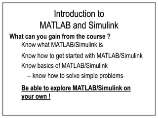
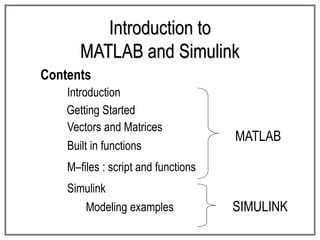
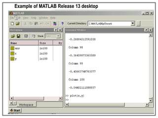
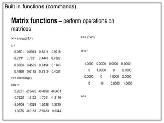
This document provides an introduction to MATLAB and Simulink. It discusses what can be gained from learning MATLAB/Simulink, including being able to solve simple problems and explore the software. The contents include an overview of built-in functions, getting started, vectors and matrices, and modeling examples in MATLAB and Simulink. It also covers M-files, script and functions, and provides examples of basic operations in MATLAB like arithmetic on matrices and accessing matrix elements.

1. An Introductory on
MATLAB and Simulink
Muhamad Zahim Sujod
zahim@kuktem.edu.my
Ext : 2312

2. Introduction to
MATLAB and Simulink
What can you gain from the course ?
Know basics of MATLAB/Simulink
– know how to solve simple problems
Know what MATLAB/Simulink is
Know how to get started with MATLAB/Simulink
Be able to explore MATLAB/Simulink on
your own !

3. Introduction to
MATLAB and Simulink
Contents
Built in functions
Getting Started
Vectors and Matrices
Introduction
Simulink
Modeling examples
MATLAB
SIMULINK
M–files : script and functions

4. Introduction
MATLAB – MATrix LABoratory
– Initially developed by a lecturer in 1970’s to help students
learn linear algebra.
– It was later marketed and further developed under
MathWorks Inc. (founded in 1984) – www.mathworks.com
– Matlab is a software package which can be used to perform
analysis and solve mathematical and engineering problems.
– It has excellent programming features and graphics capability
– easy to learn and flexible.
– Available in many operating systems – Windows, Macintosh,
Unix, DOS
– It has several tooboxes to solve specific problems.

5. Introduction
Simulink
– Used to model, analyze and simulate dynamic
systems using block diagrams.
– Fully integrated with MATLAB , easy and fast to
learn and flexible.
– It has comprehensive block library which can be
used to simulate linear, non–linear or discrete
systems – excellent research tools.
– C codes can be generated from Simulink models for
embedded applications and rapid prototyping of
control systems.

6. Getting Started
Run MATLAB from Start  Programs  MATLAB
Depending on version used, several windows appear
• For example in Release 13 (Ver 6), there are several
windows – command history, command, workspace, etc
• For Matlab Student – only command window
Command window
• Main window – where commands are entered

7. Example of MATLAB Release 13 desktop

8. Variables
– Vectors and Matrices –
ALL variables are matrices
Variables
•They are case–sensitive i.e x  X
•Their names can contain up to 31 characters
•Must start with a letter
Variables are stored in workspace
e.g. 1 x 1 4 x 1 1 x 4 2 x 4






4
2
3
9
6
5
1
2
 
7
1
2
3












3
9
2
3
 
4

9. Vectors and Matrices
 How do we assign a value to a variable?
>>> v1=3
v1 =
3
>>> i1=4
i1 =
4
>>> R=v1/i1
R =
0.7500
>>>
>>> whos
Name Size Bytes Class
R 1x1 8 double array
i1 1x1 8 double array
v1 1x1 8 double array
Grand total is 3 elements using 24 bytes
>>> who
Your variables are:
R i1 v1
>>>

10. Vectors and Matrices

















18
16
14
12
10
B
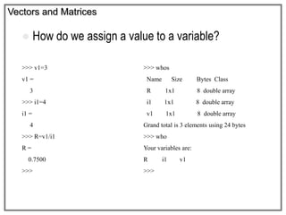
 How do we assign values to vectors?
>>> A = [1 2 3 4 5]
A =
1 2 3 4 5
>>>
>>> B = [10;12;14;16;18]
B =
10
12
14
16
18
>>>
A row vector –
values are
separated by
spaces
A column
vector –
values are
separated by
semi–colon
(;)
 
5
4
3
2
1
A 

11. Vectors and Matrices
If we want to construct a vector of, say, 100
elements between 0 and 2 – linspace
>>> c1 = linspace(0,(2*pi),100);
>>> whos
Name Size Bytes Class
c1 1x100 800 double array
Grand total is 100 elements using 800 bytes
>>>
 How do we assign values to vectors?

12. Vectors and Matrices
 How do we assign values to vectors?
If we want to construct an array of, say, 100
elements between 0 and 2 – colon notation
>>> c2 = (0:0.0201:2)*pi;
>>> whos
Name Size Bytes Class
c1 1x100 800 double array
c2 1x100 800 double array
Grand total is 200 elements using 1600 bytes
>>>

13. Vectors and Matrices
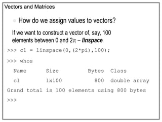
 How do we assign values to matrices ?
Columns separated by
space or a comma
Rows separated by
semi-colon
>>> A=[1 2 3;4 5 6;7 8 9]
A =
1 2 3
4 5 6
7 8 9
>>> 









9
8
7
6
5
4
3
2
1

14. Vectors and Matrices
 How do we access elements in a matrix or a vector?
Try the followings:
>>> A(2,3)
ans =
6
>>> A(:,3)
ans =
3
6
9
>>> A(1,:)
ans =
1 2 3
>>> A(2,:)
ans =
4 5 6

15. Vectors and Matrices
 Some special variables
beep
pi ()
inf (e.g. 1/0)
i, j ( )
1

>>> 1/0
Warning: Divide by zero.
ans =
Inf
>>> pi
ans =
3.1416
>>> i
ans =
0+ 1.0000i

16. Vectors and Matrices
 Arithmetic operations – Matrices
Performing operations to every entry in a matrix
Add and subtract
>>> A=[1 2 3;4 5 6;7 8
9]
A =
1 2 3
4 5 6
7 8 9
>>>
>>> A+3
ans =
4 5 6
7 8 9
10 11 12
>>> A-2
ans =
-1 0 1
2 3 4
5 6 7

17. Vectors and Matrices
 Arithmetic operations – Matrices
Performing operations to every entry in a matrix
Multiply and divide
>>> A=[1 2 3;4 5 6;7 8 9]
A =
1 2 3
4 5 6
7 8 9
>>>
>>> A*2
ans =
2 4 6
8 10 12
14 16 18
>>> A/3
ans =
0.3333 0.6667 1.0000
1.3333 1.6667 2.0000
2.3333 2.6667 3.0000

18. Vectors and Matrices
 Arithmetic operations – Matrices
Performing operations to every entry in a matrix
Power
>>> A=[1 2 3;4 5 6;7 8 9]
A =
1 2 3
4 5 6
7 8 9
>>>
A^2 = A * A
To square every element in A, use
the element–wise operator .^
>>> A.^2
ans =
1 4 9
16 25 36
49 64 81
>>> A^2
ans =
30 36 42
66 81 96
102 126 150

19. Vectors and Matrices
 Arithmetic operations – Matrices
Performing operations between matrices
>>> A=[1 2 3;4 5 6;7 8 9]
A =
1 2 3
4 5 6
7 8 9
>>> B=[1 1 1;2 2 2;3 3 3]
B =
1 1 1
2 2 2
3 3 3
A*B 



















3
3
3
2
2
2
1
1
1
9
8
7
6
5
4
3
2
1
A.*B










3
x
9
3
x
8
3
x
7
2
x
6
2
x
5
2
x
4
1
x
3
1
x
2
1
x
1










27
24
21
12
10
8
3
2
1
=
=










50
50
50
32
32
32
14
14
14

20. Vectors and Matrices
 Arithmetic operations – Matrices
Performing operations between matrices
A/B
A./B










0000
.
3
6667
.
2
3333
.
2
0000
.
3
5000
.
2
0000
.
2
0000
.
3
0000
.
2
0000
.
1
=
? (matrices singular)










3
/
9
3
/
8
3
/
7
2
/
6
2
/
5
2
/
4
1
/
3
1
/
2
1
/
1

21. Vectors and Matrices
 Arithmetic operations – Matrices
Performing operations between matrices
A^B
A.^B










729
512
343
36
25
16
3
2
1
=
??? Error using ==> ^
At least one operand must be scalar










3
3
3
2
2
2
1
1
1
9
8
7
6
5
4
3
2
1

22. Vectors and Matrices
 Arithmetic operations – Matrices
Example:
Solve for V1 and V2
10
j10
-j5
1.50o
2-90o

23. Example (cont)
(0.1 + j0.2)V1 – j0.2V2 = -j2
- j0.2V1 + j0.1V2 = 1.5
Vectors and Matrices
 Arithmetic operations – Matrices









1
.
0
j
2
.
0
j
2
.
0
j
2
.
0
j
1
.
0






2
1
V
V
= 





5
.
1
2
j
A x y
=

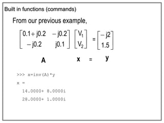
24. Example (cont)
Vectors and Matrices
 Arithmetic operations – Matrices
>>> A=[(0.1+0.2j) -0.2j;-0.2j 0.1j]
A =
0.1000+ 0.2000i 0- 0.2000i
0- 0.2000i 0+ 0.1000i
>>> y=[-2j;1.5]
y =
0- 2.0000i
1.5000
>>> x=Ay
x =
14.0000+ 8.0000i
28.0000+ 1.0000i
>>>
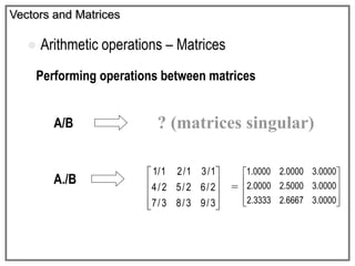
* AB is the matrix division of A into B,
which is roughly the same as INV(A)*B *

25. Example (cont)
Vectors and Matrices
 Arithmetic operations – Matrices
>>> V1= abs(x(1,:))
V1 =
16.1245
>>> V1ang= angle(x(1,:))
V1ang =
0.5191
V1 = 16.1229.7o V

26. Built in functions
(commands)
Scalar functions – used for scalars and operate
element-wise when applied to a matrix or vector
e.g. sin cos tan atan asin log
abs angle sqrt round floor
At any time you can use the command
help to get help
e.g. >>>help sin

27. Built in functions (commands)
>>> a=linspace(0,(2*pi),10)
a =
Columns 1 through 7
0 0.6981 1.3963 2.0944 2.7925 3.4907
4.1888
Columns 8 through 10
4.8869 5.5851 6.2832
>>> b=sin(a)
b =
Columns 1 through 7
0 0.6428 0.9848 0.8660 0.3420 -0.3420
-0.8660
Columns 8 through 10
-0.9848 -0.6428 0.0000
>>>

28. Built in functions (commands)
Vector functions – operate on vectors returning
scalar value
e.g. max min mean prod sum length
>>> max(b)
ans =
0.9848
>>> max(a)
ans =
6.2832
>>> length(a)
ans =
10
>>>
>>> a=linspace(0,(2*pi),10);
>>> b=sin(a);

29. Built in functions (commands)
Matrix functions – perform operations on
matrices
>>> help elmat
>>> help matfun
e.g. eye size inv det eig
At any time you can use the command
help to get help

30. Built in functions (commands)
Matrix functions – perform operations on
matrices
>>> x=rand(4,4)
x =
0.9501 0.8913 0.8214 0.9218
0.2311 0.7621 0.4447 0.7382
0.6068 0.4565 0.6154 0.1763
0.4860 0.0185 0.7919 0.4057
>>> xinv=inv(x)
xinv =
2.2631 -2.3495 -0.4696 -0.6631
-0.7620 1.2122 1.7041 -1.2146
-2.0408 1.4228 1.5538 1.3730
1.3075 -0.0183 -2.5483 0.6344
>>> x*xinv
ans =
1.0000 0.0000 0.0000 0.0000
0 1.0000 0 0.0000
0.0000 0 1.0000 0.0000
0 0 0.0000 1.0000
>>>

31. From our previous example,









1
.
0
j
2
.
0
j
2
.
0
j
2
.
0
j
1
.
0






2
1
V
V
= 





5
.
1
2
j
A x y
=
Built in functions (commands)
>>> x=inv(A)*y
x =
14.0000+ 8.0000i
28.0000+ 1.0000i

32. Built in functions (commands)
Data visualisation – plotting graphs
>>> help graph2d
>>> help graph3d
e.g. plot polar loglog mesh
semilog plotyy surf

33. Built in functions (commands)
Data visualisation – plotting graphs
Example on plot – 2 dimensional plot
Example on plot – 2 dimensional plot
>>> x=linspace(0,(2*pi),100);
>>> y1=sin(x);
>>> y2=cos(x);
>>> plot(x,y1,'r-')
>>> hold
Current plot held
>>> plot(x,y2,'g--')
>>>
Add title, labels and legend
title xlabel ylabel legend
Use ‘copy’ and ‘paste’ to add to your
window–based document, e.g. MSword
eg1_plt.m

34. Built in functions (commands)
Data visualisation – plotting graphs
0 1 2 3 4 5 6 7
-1
-0.8
-0.6
-0.4
-0.2
0
0.2
0.4
0.6
0.8
1
angular frequency (rad/s)
y1
and
y2
Example on plot
sin(x)
cos(x)
Example on plot – 2 dimensional plot
eg1_plt.m

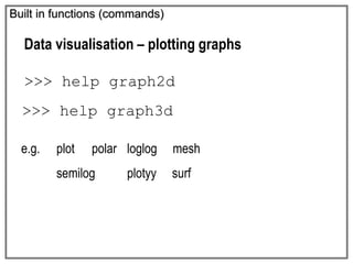
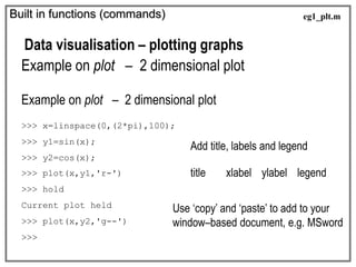
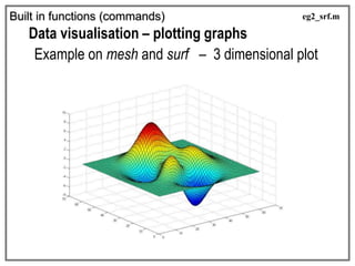
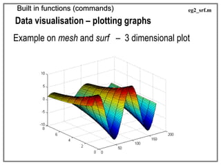
35. Built in functions (commands)
Data visualisation – plotting graphs
Example on mesh and surf – 3 dimensional plot
>>> [t,a] = meshgrid(0.1:.01:2, 0.1:0.5:7);
>>> f=2;
>>> Z = 10.*exp(-a.*0.4).*sin(2*pi.*t.*f);
>>> surf(Z);
>>> figure(2);
>>> mesh(Z);
Supposed we want to visualize a function
Z = 10e(–0.4a) sin (2ft) for f = 2
when a and t are varied from 0.1 to 7 and 0.1 to 2, respectively
eg2_srf.m

36. Built in functions (commands)
Data visualisation – plotting graphs
Example on mesh and surf – 3 dimensional plot
eg2_srf.m

37. Built in functions (commands)
Data visualisation – plotting graphs
Example on mesh and surf – 3 dimensional plot
>>> [x,y] = meshgrid(-3:.1:3,-3:.1:3);
>>> z = 3*(1-x).^2.*exp(-(x.^2) - (y+1).^2) ...
- 10*(x/5 - x.^3 - y.^5).*exp(-x.^2-y.^2) ...
- 1/3*exp(-(x+1).^2 - y.^2);
>>> surf(z);
eg3_srf.m

38. Built in functions (commands)
Data visualisation – plotting graphs
Example on mesh and surf – 3 dimensional plot
eg2_srf.m

39. Solution : use M-files
M-files :
Script and function files
When problems become complicated and require re–
evaluation, entering command at MATLAB prompt is
not practical
Collections of commands
Executed in sequence when called
Saved with extension “.m”
Script Function
User defined commands
Normally has input &
output
Saved with extension “.m”

40. M-files : script and function files (script)
At Matlab prompt type in edit to invoke M-file editor
Save this file
as test1.m
eg1_plt.m

41. M-files : script and function files (script)
To run the M-file, type in the name of the file at the
prompt e.g. >>> test1
Type in matlabpath to check the list of directories
listed in the path
Use path editor to add the path: File  Set path …
It will be executed provided that the saved file is in the
known path

42. M-files : script and function files (script)
Example – RLC circuit
Exercise 1:
Write an m–file to plot Z, Xc and XLversus
frequency for R =10, C = 100 uF, L = 0.01 H.
+
V
–
R = 10 C
L
eg4.m
eg5_exercise1.m

43. M-files : script and function files (script)
Example – RLC circuit
Total impedance is given by:
L
C X
X 
When
LC
1
o 


44. M-files : script and function files (script)
Example – RLC circuit
0 200 400 600 800 1000 1200 1400 1600 1800 2000
0
20
40
60
80
100
120
Z
Xc
Xl
eg4.m
eg5_exercise1.m

45. M-files : script and function files (script)
For a given values of C and L, plot the following versus the frequency
a) the total impedance ,
b) Xc and XL
c) phase angle of the total impedance
for 100 <  < 2000
Example – RLC circuit
+
V
–
R = 10 C
L
eg6.m

46. M-files : script and function files (script)
Example – RLC circuit
0 200 400 600 800 1000 1200 1400 1600 1800 2000
-100
-50
0
50
100
Phase
0 200 400 600 800 1000 1200 1400 1600 1800 2000
0
20
40
60
80
100
Magnitude
Mag imp
Xc
Xl
eg6.m

47.  Function is a ‘black box’ that communicates with
workspace through input and output variables.
INPUT OUTPUT
FUNCTION
– Commands
– Functions
– Intermediate variables
M-files : script and function files (function)

48. Every function must begin with a header:
M-files : script and function files (function)
function output=function_name(inputs)
Output variable
Must match the
file name
input variable

49.  Function – a simple example
function y=react_C(c,f)
%react_C calculates the reactance of a capacitor.
%The inputs are: capacitor value and frequency in hz
%The output is 1/(wC) and angular frequency in rad/s
y(1)=2*pi*f;
w=y(1);
y(2)=1/(w*c);
M-files : script and function files (function)
File must be saved to a known path with filename the same as the
function name and with an extension ‘.m’
Call function by its name and arguments
help react_C will display comments after the header

50.  Function – a more realistic example
function x=impedance(r,c,l,w)
%IMPEDANCE calculates Xc,Xl and Z(magnitude) and
%Z(angle) of the RLC connected in series
%IMPEDANCE(R,C,L,W) returns Xc, Xl and Z (mag) and
%Z(angle) at W rad/s
%Used as an example for IEEE student, UTM
%introductory course on MATLAB
if nargin <4
error('not enough input arguments')
end;
x(1) = 1/(w*c);
x(2) = w*l;
Zt = r + (x(2) - x(1))*i;
x(3) = abs(Zt);
x(4)= angle(Zt);
M-files : script and function files (function) impedance.m

51. We can now add our function to a script M-file
R=input('Enter R: ');
C=input('Enter C: ');
L=input('Enter L: ');
w=input('Enter w: ');
y=impedance(R,C,L,w);
fprintf('n The magnitude of the impedance at %.1f
rad/s is %.3f ohmn', w,y(3));
fprintf('n The angle of the impedance at %.1f rad/s is
%.3f degreesnn', w,y(4));
M-files : script and function files (function) eg7_fun.m

52. Simulink
Used to model, analyze and simulate dynamic
systems using block diagrams.
Provides a graphical user interface for constructing
block diagram of a system – therefore is easy to use.
However modeling a system is not necessarily easy !

53. Simulink
Model – simplified representation of a system – e.g. using
mathematical equation
We simulate a model to study the behavior of a system –
need to verify that our model is correct – expect results
Knowing how to use Simulink or MATLAB does not
mean that you know how to model a system

54. Simulink
Problem: We need to simulate the resonant circuit
and display the current waveform as we change the
frequency dynamically.
+
v(t) = 5 sin t
–
i 10  100 uF
0.01 H
Varies 
from 0 to
2000 rad/s
Observe the current. What do we expect ?
The amplitude of the current waveform will become
maximum at resonant frequency, i.e. at  = 1000 rad/s

55. Simulink
How to model our resonant circuit ?
+
v(t) = 5 sin t
–
i 10  100 uF
0.01 H



 idt
C
1
dt
di
L
iR
v
Writing KVL around the loop,

56. Simulink
LC
i
dt
i
d
L
R
dt
di
dt
dv
L
1
2
2



Differentiate wrt time and re-arrange:
Taking Laplace transform:
LC
I
I
s
sI
L
R
L
sV 2












LC
1
s
L
R
s
I
L
sV 2

57. Simulink
Thus the current can be obtained from the voltage:













LC
1
s
L
R
s
)
L
/
1
(
s
V
I
2
LC
1
s
L
R
s
)
L
/
1
(
s
2


V I

58. Simulink
Start Simulink by typing simulink at Matlab prompt
Simulink library and untitled windows appear
It is here where we
construct our model.
It is where we
obtain the blocks to
construct our model

59. Simulink
Constructing the model using Simulink:
‘Drag and drop’ block from the Simulink library
window to the untitled window
1
s+1
Transfer Fcn
simout
To Workspace
Sine Wave

60. Simulink
Constructing the model using Simulink:
LC
1
s
L
R
s
)
L
/
1
(
s
2

 6
2
10
1
s
1000
s
)
100
(
s



100s
s +1000s+1e6
2
Transfer Fcn
v
To Workspace1
i
To Workspace
Sine Wave

61. Simulink
We need to vary the frequency and observe the current
100s
s +1000s+1e6
2
Transfer Fcn1
v
To Workspace3
w
To Workspace2
i
To Workspace
Ramp
s
1
Integrator
sin
Elementary
Math
Dot Product3
Dot Product2
1000
Constant
5
Amplitude
eg8_sim.mdl
…From initial problem definition, the input is 5sin(ωt).
You should be able to decipher why the input works, but
you do not need to create your own input subsystems of
this form.

62. Simulink
0 0.1 0.2 0.3 0.4 0.5 0.6 0.7 0.8 0.9 1
-1
-0.5
0
0.5
1
0 0.1 0.2 0.3 0.4 0.5 0.6 0.7 0.8 0.9 1
-5
0
5

63. Simulink
The waveform can be displayed using scope – similar
to the scope in the lab
100s
s +1000s+1e6
2
Transfer Fcn
0.802
Slider
Gain
Scope
s
1
Integrator
sin
Elementary
Math
Dot Product2
5
Constant1
2000
Constant
eg9_sim.mdl

64. Reference
 Internet – search engine
 Mastering MATLAB 6 (Prentice Hall)
– Duane Hanselman
– Bruce Littlefield