The document provides an introduction to MATLAB and Simulink through a presentation. It discusses what MATLAB and Simulink are, their basic functions and capabilities, and how to get started using them. The presentation covers topics such as vectors, matrices, plotting, control structures, M-files, and writing user-defined functions. The goal is to help attendees gain basic knowledge of MATLAB/Simulink and be able to explore them on their own.

1. “MATLAB
EXPLORATION”
(Place to visualize your thoughts)
Presentation By
Mr. ReddyPrasad Reddivari,
Assistant Professor
Department of Electrical and Electronics Engineering
Sri Venkateshwara College of Engineering
Bengaluru, Karnataka-562157
Tel: 9494747497
E-Mail: reddytnp.244@gmail.com.
Website: www.reddyprasad.yolasite.com
MATLAB/SIMULINK for Engineering applications

2. Introduction to Matlab

3. Introduction to
MATLAB and Simulink
What can you gain from the course ?
Know basics of MATLAB/Simulink
– know how to solve simple problems
Know what MATLAB/Simulink is
Know how to get started with MATLAB/Simulink
Be able to explore MATLAB/Simulink onBe able to explore MATLAB/Simulink on
your own !your own !

4. Introduction to
MATLAB and Simulink
Contents
Built in functions
Getting Started
Vectors and Matrices
Introduction
Simulink
Modeling examples
MATLAB
SIMULINK
M–files : script and functions

5. Introduction
MATLAB – MATrix LABoratory
 Initially developed by a lecturer in 1970’s to help students
learn linear algebra.
 It was later marketed and further developed under MathWorks
Inc. (founded in 1984) – www.mathworks.com
 Matlab is a software package which can be used to perform
analysis and solve mathematical and engineering problems.
 It has excellent programming features and graphics capability
– easy to learn and flexible.
 Available in many operating systems – Windows, Macintosh,
Unix, DOS
 It has several tooboxes to solve specific problems.

6. Outline:
 What is Matlab?
 Matlab Screen
 Variables, array, matrix, indexing
 Operators (Arithmetic, relational, logical )
 Display Facilities
 Flow Control
 Using of M-File
 Writing User Defined Functions
 plotting

7. What is Matlab?
 Matlab is basically a high level language
which has many specialized toolboxes for
making things easier for us
 How high?
Assembly
High Level
Languages such as
C, Pascal etc.
Matlab

8. What are we interested in?
 Matlab is too broad for our purposes in this
course.
 The features we are going to require is
Matlab
Command
Line
m-files
functions
mat-files
Command execution
like DOS command
window
Series of
Matlab
commands
Input
Output
capability
Data
storage/
loading

9. Matlab Screen
 Command Window
 type commands
 Current Directory
 View folders and m-files
 Workspace
 View program variables
 Double click on a variable
to see it in the Array Editor
 Command History
 view past commands
 save a whole session
using diary

10. Variables
 No need for types. i.e.,
 All variables are created with double precision unless
specified and they are matrices.
 After these statements, the variables are 1x1 matrices
with double precision
int a;
double b;
float c;
Example:
>>x=5;
>>x1=2;

11. Mathematical Operators
 Mathematical Operators:
 Add: +
 Subtract: -
 Divide: ./
 Multiply: .*
 Power: .^ (e.g. .^2 means squared)
 You can use round brackets to specify the order in
which operations will be performed
 Note that preceding the symbol / or * or ^ by a ‘.’
means that the operator is applied between pairs of
corresponding elements of vectors of matrices
11

12. Logical Operators
You can use Logical Indexing to find data that
conforms to some limitations
Logical Operators:
 Greater Than: >
 Less Than: <
 Greater Than or Equal To: >=
 Less Than or Equal To: <=
 Is Equal: ==
 Not Equal To: ~=
12

13. Boolean Operators
Boolean Operators:
 AND: &
 OR: |
 NOT: ~
 Connects two logical expressions together
13

14. Special functions
 There are a number of special functions that provide
useful constants
 pi = 3.14159265….
 i or j = square root of -1
 Inf = infinity
 NaN = not a number

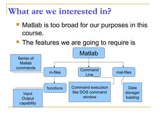
15. Array, Matrix
 a vector x = [1 2 5 1]
x =
1 2 5 1
 a matrix x = [1 2 3; 5 1 4; 3 2 -1]
x =
1 2 3
5 1 4
3 2 -1
 transpose y = x’ y =
1
2
5
1

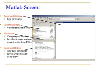
16. Long Array, Matrix
 t =1:10
t =
1 2 3 4 5 6 7 8 9 10
 k =2:-0.5:-1
k =
2 1.5 1 0.5 0 -0.5 -1
 B = [1:4; 5:8]
x =
1 2 3 4
5 6 7 8

17. Generating Vectors from functions
 zeros(M,N) MxN matrix of zeros
 ones(M,N) MxN matrix of ones
 rand(M,N) MxN matrix of uniformly
distributed random
numbers on (0,1)
x = zeros(1,3)
x =
0 0 0
x = ones(1,3)
x =
1 1 1
x = rand(1,3)
x =
0.9501 0.2311 0.6068

18. Matrix Index
 The matrix indices begin from 1 (not 0 (as in C))
 The matrix indices must be positive integer
Given:
A(-2), A(0)
Error: ??? Subscript indices must either be real positive integers or logicals.
A(4,2)
Error: ??? Index exceeds matrix dimensions.

19. Matrix Reference
Consider a 4-by-3 matrix
How is it arranged in memory?
A(1,1)
A(2,1)
A(3,1)
A(4,1)
A(1,2)
A(2,2)
A(3,2)
A(4,2)
A(1,3)
A(2,3)
A(3,3)
A(4,3)
1
2
3
4
5
6
7
8
9
10
11
12
 For 2-d double array, to move through memory sequentially
– the first index changes the fastest, and
– the second index changes the slowest
 conversion: ind2sub, sub2ind
1st
element
2nd
element
3rd
4th
5th
6th
7th
8th
9th
10th
11th
12th
full index
linear index
19

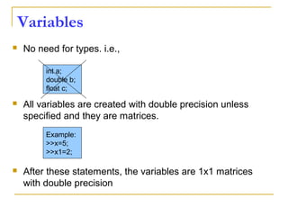
20. Concatenation of Matrices
 x = [1 2], y = [4 5], z=[ 0 0]
A = [ x y]
1 2 4 5
B = [x ; y]
1 2
4 5
C = [x y ;z]
Error:
??? Error using ==> vertcat CAT arguments dimensions are not consistent.

21. Operators (arithmetic)
+ addition
- subtraction
* multiplication
/ division
^ power
‘ complex conjugate transpose

22. Matrices Operations
Given A and B:
Addition Subtraction Product Transpose

23. Operators (Element by Element)
.* element-by-element multiplication
./ element-by-element division
.^ element-by-element power

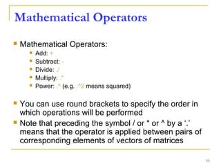
24. The use of “.” – “Element” Operation
K= x^2
Erorr:
??? Error using ==> mpower Matrix must be square.
B=x*y
Erorr:
??? Error using ==> mtimes Inner matrix dimensions must agree.
A = [1 2 3; 5 1 4; 3 2 1]
A =
1 2 3
5 1 4
3 2 -1
y = A(3 ,:)
y=
3 4 -1
b = x .* y
b=
3 8 -3
c = x . / y
c=
0.33 0.5 -3
d = x .^2
d=
1 4 9
x = A(1,:)
x=
1 2 3

25. Basic Task: Plot the function sin(x)
between 0≤x≤4π
 Create an x-array of 100 samples between 0
and 4π.
 Calculate sin(.) of the x-array
 Plot the y-array
>>x=linspace(0,4*pi,100);
>>y=sin(x);
>>plot(y)
0 10 20 30 40 50 60 70 80 90 100
-1
-0.8
-0.6
-0.4
-0.2
0
0.2
0.4
0.6
0.8
1

26. Plot the function e-x/3
sin(x) between
0≤x≤4π
 Create an x-array of 100 samples between 0
and 4π.
 Calculate sin(.) of the x-array
 Calculate e-x/3
of the x-array
 Multiply the arrays y and y1
>>x=linspace(0,4*pi,100);
>>y=sin(x);
>>y1=exp(-x/3);
>>y2=y*y1;

27. Plot the function e-x/3
sin(x) between
0≤x≤4π
 Multiply the arrays y and y1 correctly
 Plot the y2-array
>>y2=y.*y1;
>>plot(y2)
0 10 20 30 40 50 60 70 80 90 100
-0.3
-0.2
-0.1
0
0.1
0.2
0.3
0.4
0.5
0.6
0.7

28. Display Facilities
 plot(.)
 stem(.)
Example:
>>x=linspace(0,4*pi,100);
>>y=sin(x);
>>plot(y)
>>plot(x,y)
Example:
>>stem(y)
>>stem(x,y)
0 10 20 30 40 50 60 70 80 90 100
-0.3
-0.2
-0.1
0
0.1
0.2
0.3
0.4
0.5
0.6
0.7
0 10 20 30 40 50 60 70 80 90 100
-0.3
-0.2
-0.1
0
0.1
0.2
0.3
0.4
0.5
0.6
0.7

29. Display Facilities
 title(.)
 xlabel(.)
 ylabel(.)
>>title(‘This is the sinus function’)
>>xlabel(‘x (secs)’)
>>ylabel(‘sin(x)’)
0 10 20 30 40 50 60 70 80 90 100
-1
-0.8
-0.6
-0.4
-0.2
0
0.2
0.4
0.6
0.8
1
This is the sinus function
x (secs)
sin(x)

30. Operators (relational, logical)
 == Equal to
 ~= Not equal to
 < Strictly smaller
 > Strictly greater
 <= Smaller than or equal to
 >= Greater than equal to
 & And operator
 | Or operator

31. Flow Control
 if
 for
 while
 break
 ….

32. Control Structures
 If Statement Syntax
if (Condition_1)
Matlab Commands
elseif (Condition_2)
Matlab Commands
elseif (Condition_3)
Matlab Commands
else
Matlab Commands
end
Some Dummy Examples
if ((a>3) & (b==5))
Some Matlab Commands;
end
if (a<3)
Some Matlab Commands;
elseif (b~=5)
Some Matlab Commands;
end
if (a<3)
Some Matlab Commands;
else
Some Matlab Commands;
end

33. Control Structures
 For loop syntax
for i=Index_Array
Matlab Commands
end
Some Dummy Examples
for i=1:100
Some Matlab Commands;
end
for j=1:3:200
Some Matlab Commands;
end
for m=13:-0.2:-21
Some Matlab Commands;
end
for k=[0.1 0.3 -13 12 7 -9.3]
Some Matlab Commands;
end

34. Control Structures
 While Loop Syntax
while (condition)
Matlab Commands
end
Dummy Example
while ((a>3) & (b==5))
Some Matlab Commands;
end

35. Use of M-File
Click to create
a new M-File
• Extension “.m”
• A text file containing script or function or program to run

36. Use of M-File
If you include “;” at the
end of each statement,
result will not be shown
immediately
Save file as Denem430.m

37. Solution : use M-files
M-files :
Script and function files
When problems become complicated and require re–
evaluation, entering command at MATLAB prompt is
not practical
Collections of commands
Executed in sequence when called
Saved with extension “.m”
Script Function
User defined commands
Normally has input & output
Saved with extension “.m”

38.  Function is a ‘black box’ that communicates with
workspace through input and output variables.
INPUT OUTPUTFUNCTION
– Commands
– Functions
– Intermediate variables
M-files : script and function files (function)

39. Every function must begin with a header:
M-files : script and function files (function)
function output=function_name(inputs)
Output variable
Must match the file
name
input variable

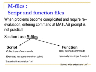
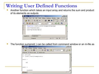
40. Writing User Defined Functions
 Functions are m-files which can be executed by
specifying some inputs and supply some desired outputs.
 The code telling the Matlab that an m-file is actually a
function is
 You should write this command at the beginning of the
m-file and you should save the m-file with a file name
same as the function name
function out1=functionname(in1)
function out1=functionname(in1,in2,in3)
function [out1,out2]=functionname(in1,in2)

41. Writing User Defined Functions
 Examples
 Write a function : out=squarer (A, ind)
 Which takes the square of the input matrix if the input
indicator is equal to 1
 And takes the element by element square of the input
matrix if the input indicator is equal to 2
Same Name

42. Writing User Defined Functions
 Another function which takes an input array and returns the sum and product
of its elements as outputs
 The function sumprod(.) can be called from command window or an m-file as

43. Notes:
 “%” is the neglect sign for Matlab (equaivalent
of “//” in C). Anything after it on the same line
is neglected by Matlab compiler.
 Sometimes slowing down the execution is
done deliberately for observation purposes.
You can use the command “pause” for this
purpose
pause %wait until any key
pause(3) %wait 3 seconds

44. Useful Commands
 The two commands used most by Matlab
users are
>>help functionname
>>lookfor keyword

45. Plotting
45

46. Plotting
 The plot function can be used in different ways:
>> plot(data)
>> plot(x, y)
>> plot(data, ‘r.-’)
 In the last example the line style is defined
Colour: r, b, g, c, k, y etc.
Point style: . + * x o > etc.
Line style: - -- : .-
 Type ‘help plot’ for a full list of the options
46

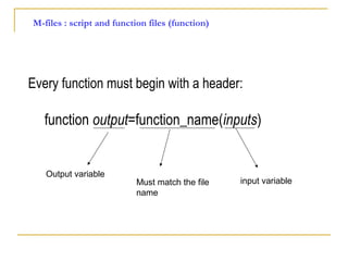
47. Plotting
 A basic plot
>> x = [0:0.1:2*pi]
>> y = sin(x)
>> plot(x, y, ‘r.-’)
47
0 1 2 3 4 5 6 7
-1
-0.8
-0.6
-0.4
-0.2
0
0.2
0.4
0.6
0.8
1

48. Plotting
 Plotting a matrix
 MATLAB will treat each column as a different set of data
48
1 2 3 4 5 6 7 8 9 10
0.1
0.2
0.3
0.4
0.5
0.6
0.7
0.8
0.9

49. Plotting
 Some other functions that are helpful to create plots:
 hold on and hold off
 title
 legend
 axis
 xlabel
 ylabel
49

50. Plotting
>> x = [0:0.1:2*pi];
>> y = sin(x);
>> plot(x, y, 'b*-')
>> hold on
>> plot(x, y*2, ‘r.-')
>> title('Sin Plots');
>> legend('sin(x)', '2*sin(x)');
>> axis([0 6.2 -2 2])
>> xlabel(‘x’);
>> ylabel(‘y’);
>> hold off
50
0 1 2 3 4 5 6
-2
-1.5
-1
-0.5
0
0.5
1
1.5
2
Sin Plots
x
y
sin(x)
2*sin(x)

51. Plotting
 Plotting data
>> results = rand(10, 3)
>> plot(results, 'b*')
>> hold on
>> plot(mean(results, 2), ‘r.-’)
51

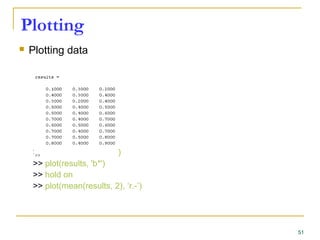
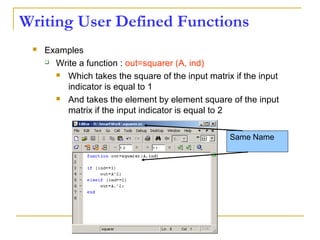
52. Plotting
Error bar plot
>> errorbar(mean(data, 2), std(data, [], 2))
52
0 2 4 6 8 10 12
0.1
0.2
0.3
0.4
0.5
0.6
0.7
0.8
0.9
1
Mean test results with error bars

53. Plotting
 You can close all the current plots using ‘close all’
53

54. Questions
 ?
 ?
 ?
 ?
 ?

55. Thank You…