Download to read offline


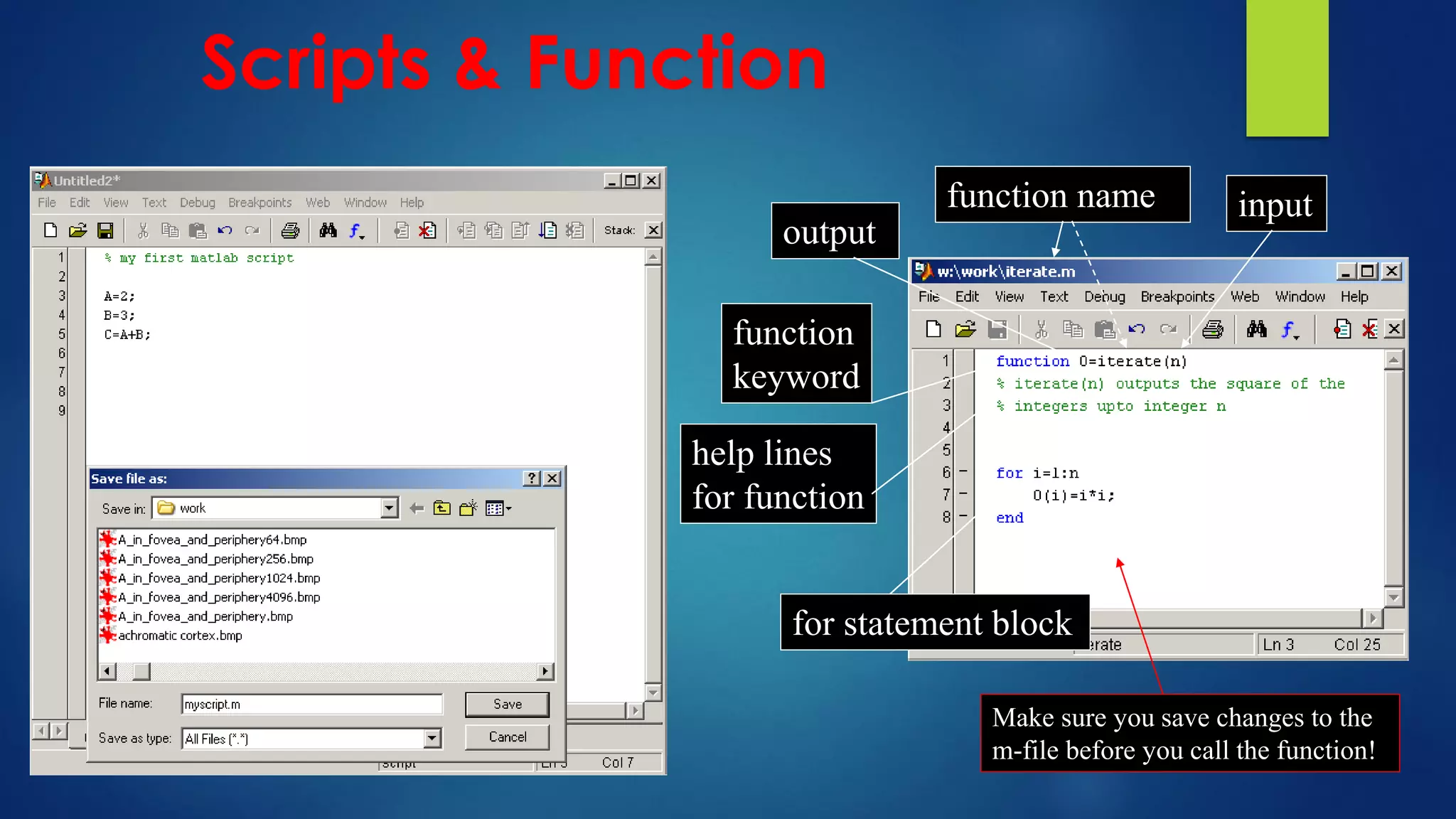
![MATLAB Array
An array is a collection of data values organized into rows and columns.
When the array has only one dimension (either a row or a column), it is known as a vector.
While a two or more dimensional array is known as a matrix.
A = [1 2 3 4 5] %A is a vector
B = [1 2 3; 4 5 6; 7 8 9] % B is a matrix
C = ‘Hello’ % C is a string array](https://image.slidesharecdn.com/matlabseminar-210504121906/75/Introduction-to-MATLAB-23-2048.jpg)
![Scalars:-
A scalars is a (1x1) matrix containing a single element only.
A scalar does not need any square brackets
P = 10
Vectors:-
Vectors are two type 1)- Row vector and 2) Column vector
All the elements of a row vector are separated by blank space or commas and are
enclosed in square brackets.
All the elements of a column are separated by semicolon.
Q = [1,2,3] / [1 2 3] – row
P = [1; 2; 3] - column
Vectors and Matrices](https://image.slidesharecdn.com/matlabseminar-210504121906/75/Introduction-to-MATLAB-25-2048.jpg)
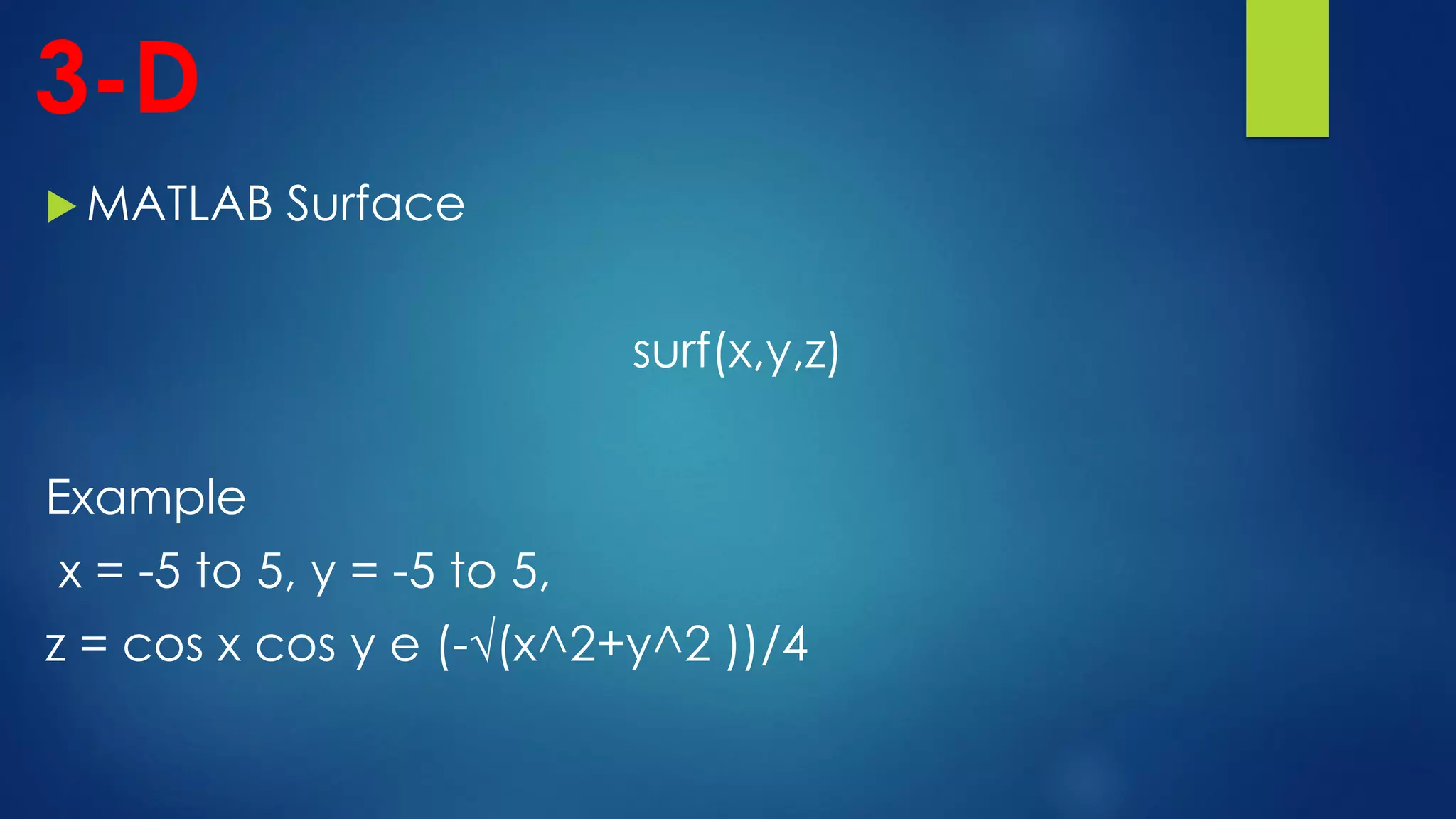

![Polynomial Functions
MATLAB performs polynomial operations.
P(x) = x4 + 7x3 - 5x + 9
Solution of this equation at 1, 9, 19 ,21 etc.
P = [1 7 0 -5 9]
x = 1
polycal(P,x)](https://image.slidesharecdn.com/matlabseminar-210504121906/75/Introduction-to-MATLAB-36-2048.jpg)


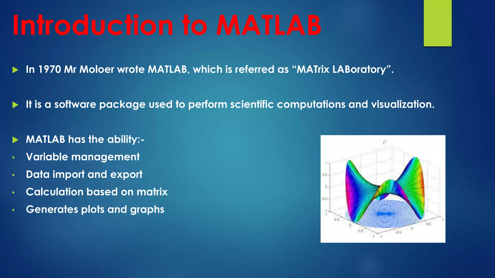
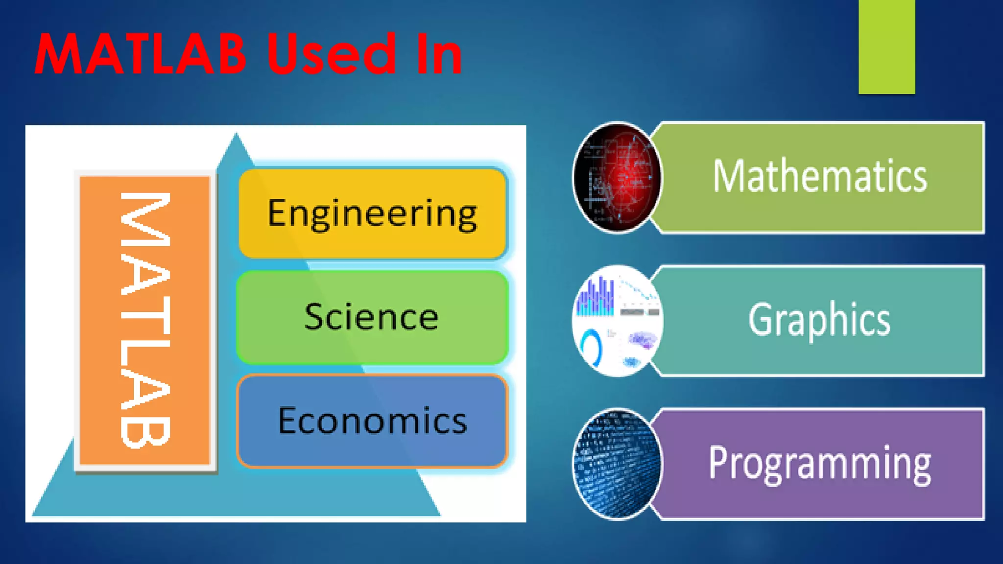
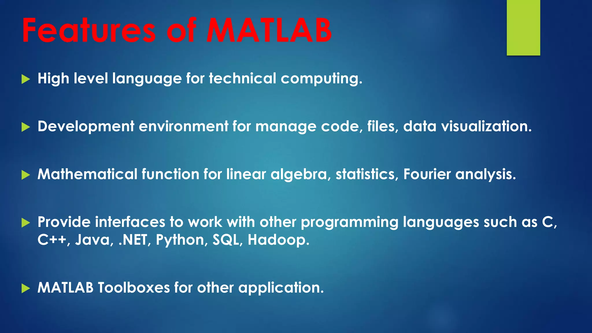
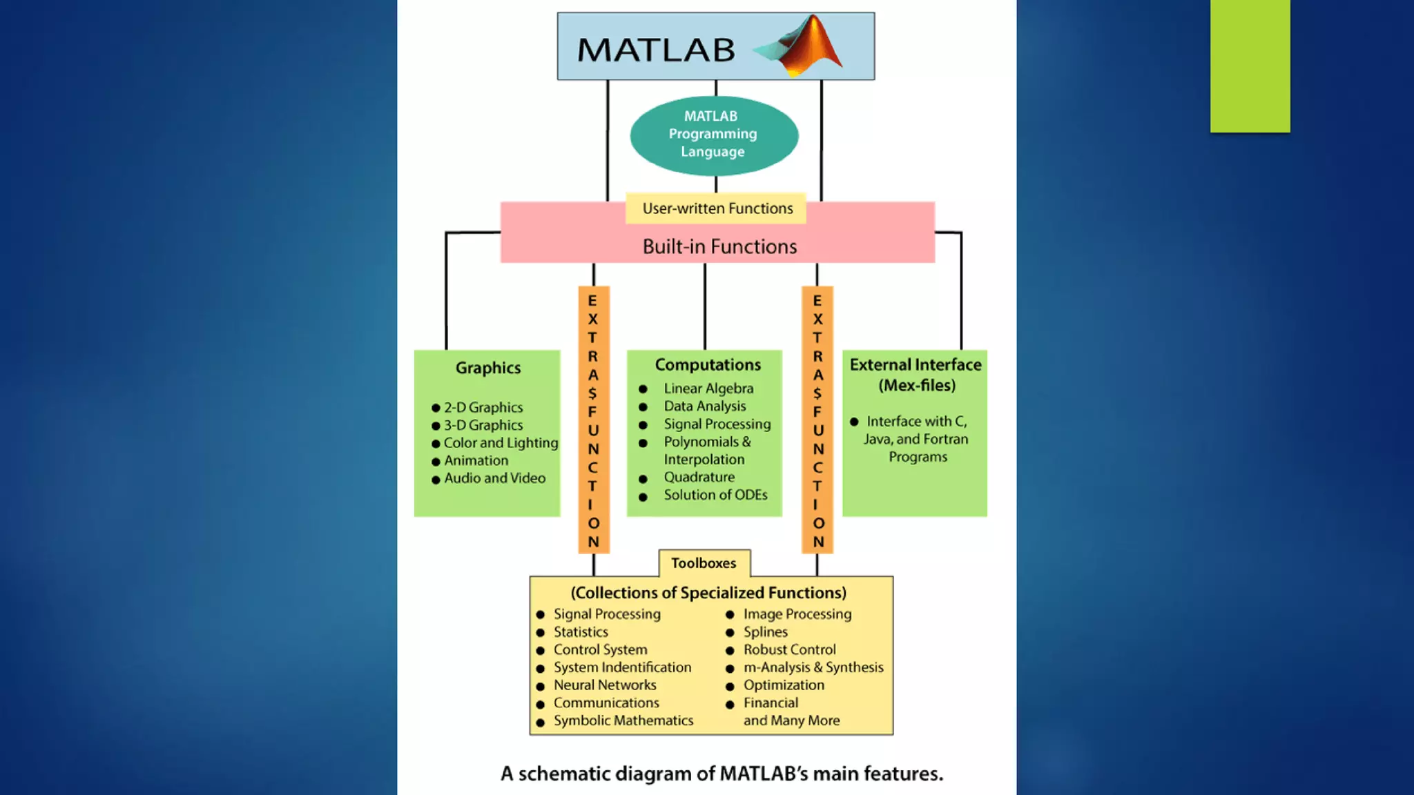
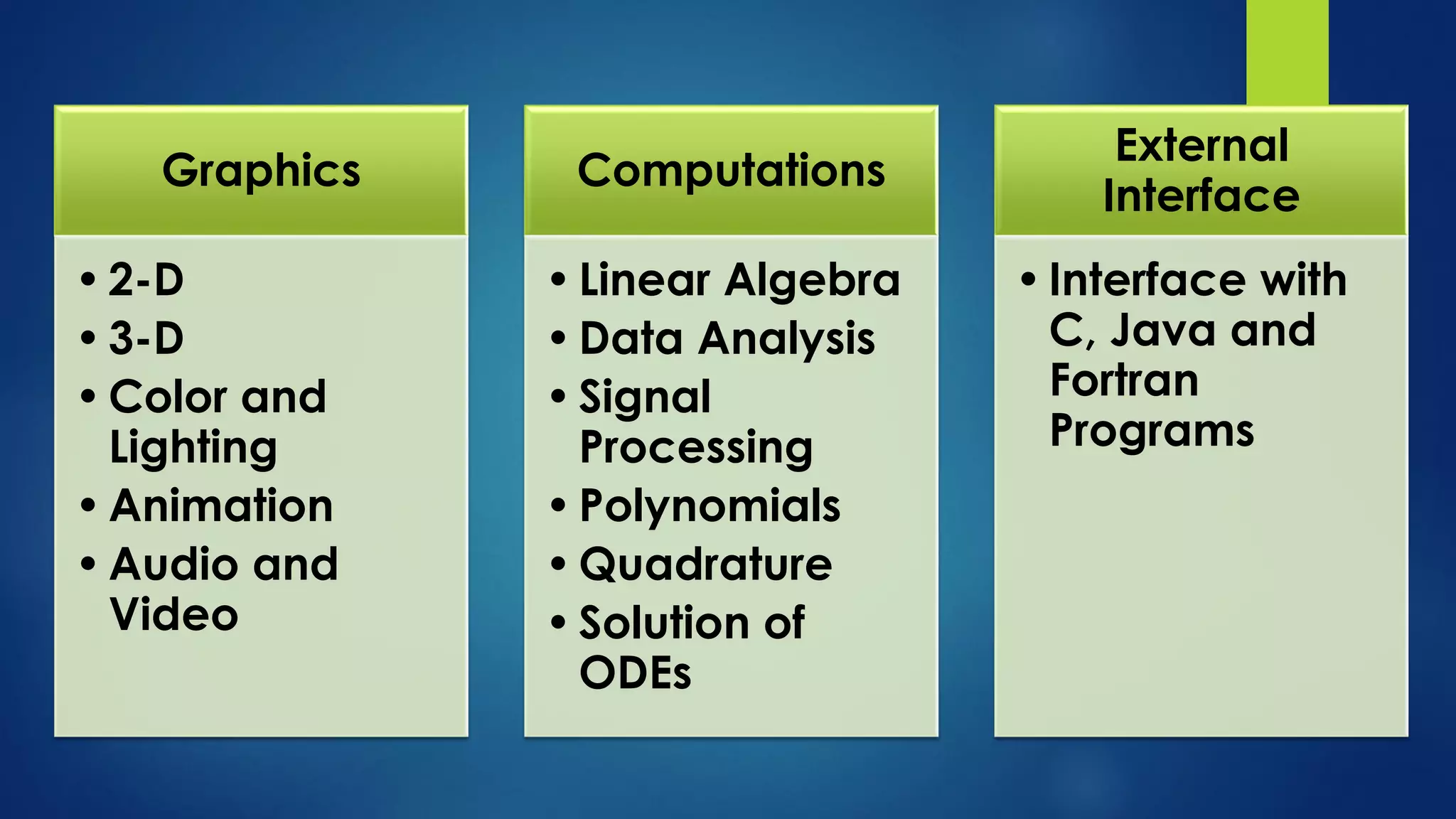
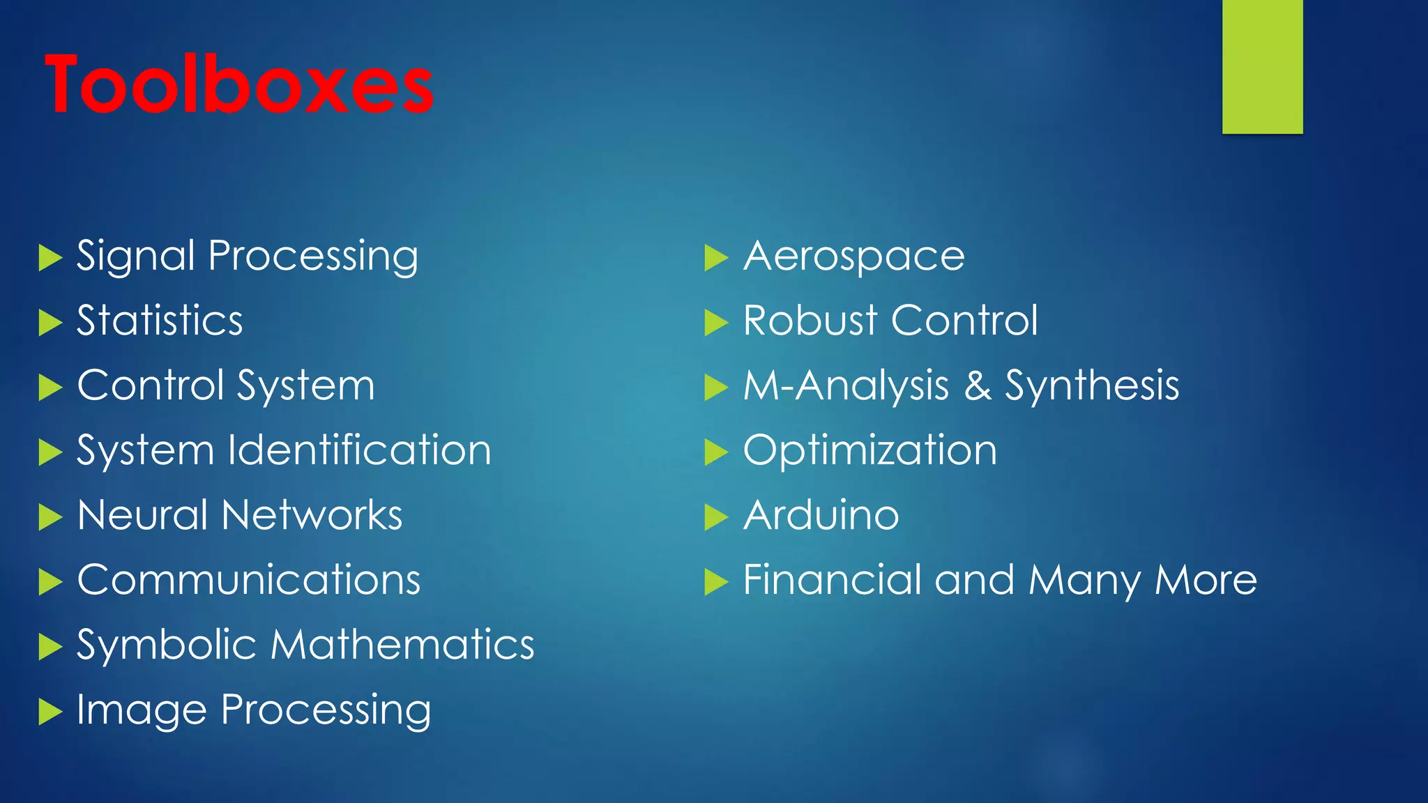
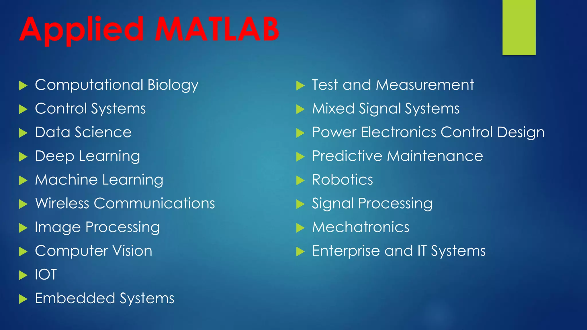
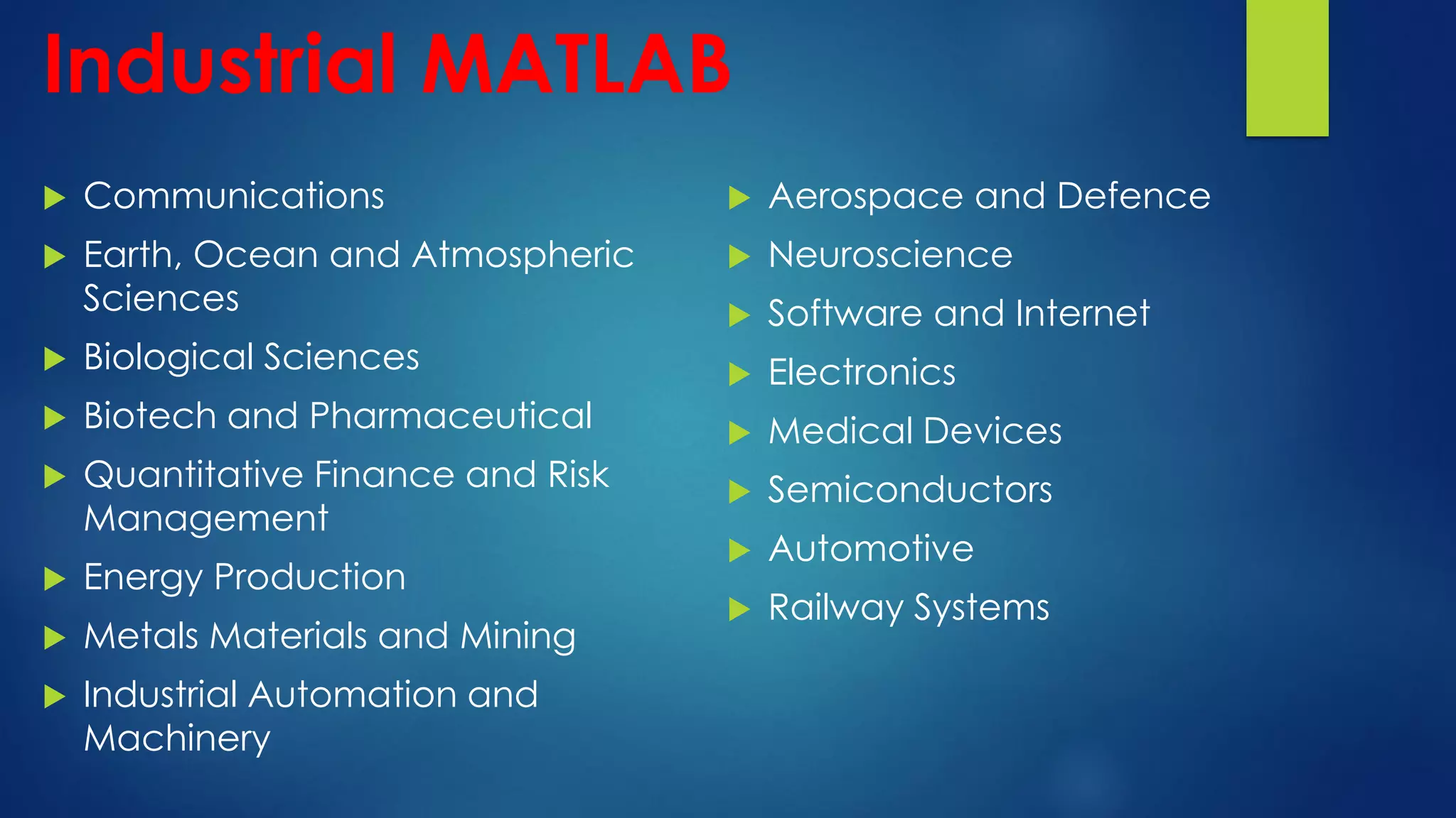
This document provides an overview of MATLAB, including what it is, its features, toolboxes, applications, and how to perform various tasks. MATLAB is a numerical computing environment and programming language used for algorithm development, data analysis, and visualization. It allows matrix operations, plotting of functions and data, implementation of algorithms, creation of user interfaces, and interfacing with programs in other languages. The document describes MATLAB's various components, data types, commands, and how to work with matrices, arrays, plots, and other mathematical functions. It also outlines uses of MATLAB in domains like signal processing, control systems, image processing, and more.