Mathematical Model of Varicella Zoster Virus - Abbie Jakubovic

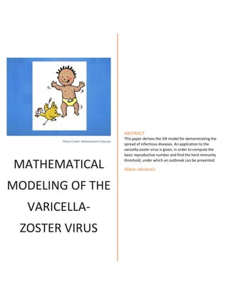
Photo Credit: Mohammed A Qazzaz
MATHEMATICAL
MODELING OF THE
VARICELLA-
ZOSTER VIRUS
ABSTRACT
This paper derives the SIR model for demonstrating the
spread of infectious diseases. An application to the
varicella-zoster virus is given, in order to compute the
basic reproductive number and find the herd immunity
threshold, under which an outbreak can be prevented.
Abbie Jakubovic

of 28
Abbie Jakubovic
Contents
Introduction ..................................................................................................................................................3
Notation and Terminology............................................................................................................................4
The S-I-R Model.............................................................................................................................................5
Applying the SIR Model to the Varicella-Zoster Virus (VZV).........................................................................9
Background ...............................................................................................................................................9
Demonstration of SIR Model for Varicella in Non-Vaccinated Population.............................................10
Variation of the S-I-R Model to Include Vaccination ..................................................................................15
Background .............................................................................................................................................15
Basic Reproductive Ratio ........................................................................................................................16
Herd Immunity........................................................................................................................................18
Estimation of R0 and Vaccination Threshold...........................................................................................22
Conclusions .................................................................................................................................................23
Bibliography ................................................................................................................................................25
Appendix A – Data Table for Varicella Outbreak with 65% Infection Rate.................................................26
Appendix B - Data Table for Varicella Outbreak with 85% Infection Rate..................................................27
Appendix C – Effects of Infection Rate Estimates on the SIR Model ..........................................................28

of 28
Abbie Jakubovic
Introduction
The annals of history are replete with staggering accounts of disease outbreak, from the
seemingly innocuous common cold to the most deadly plagues that threatened to destroy
entire populations. The 21st century is cognizant of epidemics of the past, such as the
approximately 75 million people who perished during the black plague, while battling current
epidemics such as HIV/AIDS, the swine flu outbreak of 2009 or the current Zika virus. Although
in the past an epidemic outbreak could be considered a death sentence for large segments of a
population, modern mathematics plays a pivotal role in identifying solutions in both treatment
and prevention of an outbreak. It has been discerned from collected data that epidemics take
on typical patterns. For example, the 1906 plague on the island of Bombay took on a slightly
skewed bell shape, with the number of deaths per week reaching its highest levels between 15
to 20 weeks from the start of the outbreak in December of the previous year. (Kermack and
McKendrick) Accordingly, the goal of mathematical epidemiology is to identify trends and
patterns in order to uncover the mechanisms that cause such events and describe them in a
Figure 1 Plague of Bombay, 1906. Credit: Kermack and McKendrick pg. 714

of 28
Abbie Jakubovic
rational manner. (Iannelli) This paper will explore some of the basic models of epidemics and
the effects of mass vaccination, known as herd immunity, with respect to the treatment and
prevention of an outbreak.
Notation and Terminology
Before introducing the basic S-I-R model as expressed by Kermack and McKendrick, it
would be prudent to briefly state the three epidemiological classes that will be used for the
basic SIR and SIS models as well as the notation for the rates at which individuals in the
population may move from one class to another. The notation presented here follows that of
Iannelli’s lectures.
 𝑆(𝑡) denotes the number of individuals in a population which are susceptible to the
disease in question at time t.
 𝐼(𝑡) denotes those infected and who are able to transmit the disease to other
individuals via contact at time t.
 𝑅(𝑡) refers to those individuals who have been removed from the population at time t,
either through recovery and achievement of immunity or through death.
 𝑁(𝑡) = 𝑆(𝑡) + 𝐼(𝑡) + 𝑅(𝑡), which is the total population at time t.
 𝜆(𝑡) is defined as the “force of infection” or the rate at which susceptible individuals become
infected.
 𝛾(𝑡) is defined as the “removal rate” meaning the rate at which infected individuals either
recover or die.

of 28
Abbie Jakubovic
 It should be noted that although “removal” can be defined either through recovery or
death, in the simple models the possibility of death is ignored and the total population is
assumed to be constant. (Iannelli)
The S-I-R Model
The SIR model is presented by Kermack and McKendrick as one or more infected individuals
being introduced into a population of individuals who are susceptible to the disease under discussion.
The disease is spread via contact between the infected and the susceptible, whereby each infected
person runs the course of the sickness after which the individual is becomes removed, either through
recovery and the attainment of immunity, or death. (Kermack and McKendrick) In the simple model, the
possibility of death is ignored, although death is a reality during an epidemic, in order to keep the total
population constant. In this vein, we also assume that there are no births or changes to demographic
dynamics during the course of the outbreak. (Iannelli) Individuals who are susceptible become infected
at a specified rate which is defined as
𝜆(𝑡) =
𝐼(𝑡)
𝑁(𝑡)
𝑐𝑥
where
c = number of contacts within the time unit,
x = infectiveness of a single contact.
The factor
𝐼(𝑡)
𝑁(𝑡)
is the probability that the contacted individual is actually infected, and this is
multiplied by the number of contacts the susceptible individuals have with infectives within the time
interval and further multiplied by the ability for that contact to impart the disease. This is referred to as
the “force of infection”.

of 28
Abbie Jakubovic
The second parameter of the SIR model, the removal rate is assumed to be a constant, defined
as
𝛾(𝑡) = 𝛾 =
1
𝜏
with 𝜏 being the average duration of the infection. Thus, an individual in the population who
begins as susceptible may become infected via the parameter (t) and will subsequently become
removed through (t).
It is important to mention the underlying assumptions of the SIR model. First, the model
assumes that everybody in the population is active and mixes together homogeneously, so that
the probability of any single contact being with an infected individual is
𝐼(𝑡)
𝑁(𝑡)
. Furthermore, the
contact rate is independent of the size of the population and the infectiveness of every contact
is equal. With respect to the removal rate, it is assumed that the progression of the disease is
the same in every individual, regardless of age, general health and other factors. Being that 𝛾 is
a constant which measures the average fraction of infected individuals in the time unit, a given
group of infected people will decrease exponentially. Finally, in the single epidemic outbreak it
The S-I-R Model

of 28
Abbie Jakubovic
is assumed that there are no shifts in demographics, births or deaths during the time interval of
the epidemic, even deaths caused by the disease. (Iannelli)
Under these assumptions, Iannelli describes the occurrence of a disease imparting
immunity by the following system of equations.
{
𝑆′(𝑡) = −𝜆(𝑡)𝑆(𝑡)
𝐼′(𝑡) = 𝜆(𝑡)𝑆(𝑡) − 𝛾𝐼(𝑡)
𝑅′(𝑡) = 𝛾𝐼(𝑡)
𝑆(0) = 𝑆0
𝐼(0) = 𝐼0
𝑅(0) = 𝑅0
where we assume that 𝑆(0) > 0, 𝐼(0) > 0 and 𝑅(0) ≥ 0. The susceptibility differential,
representing the rate of change in the number of susceptible individuals at time t, is
understandably negative. As time is increased, the number of susceptibles will decrease as
people become infected and eventually removed. The rate of change is then the number of
susceptible individuals multiplied by the force of infection. It then follows that the infective
differential is made up of the number of susceptibles who became infected less those who have
been removed. Finally, the rate of change in the number of those removed would be the
removal rate multiplied by the number infected at that time. This system of equations implies
our initial assumption that the total population remains constant by noting that
𝑆′(𝑡) + 𝐼′(𝑡) + 𝑅′(𝑡) = 0 𝑠𝑢𝑐ℎ 𝑡ℎ𝑎𝑡
𝑁(𝑡) = 𝑆0 + 𝐼0 + 𝑅0 = 𝑁,
which is a parameter of the model, in the denominator of the force of infection.
Iannelli makes a number of important observations from the above equations. First we
note that 𝑆′(𝑡) < 0, so that S(t) is a decreasing function as t increases. Further he notes that

of 28
Abbie Jakubovic
𝑑
𝑑𝑡
[𝑆(𝑡) + 𝐼(𝑡)] = −𝛾𝐼(𝑡) < 0
and that
𝛾 ∫ 𝐼(𝑠)𝑑𝑠
𝑡
0
= 𝑅(𝑡) = 𝑁 − 𝑆(𝑡) − 𝐼(𝑡) ≤ 𝑁,
so that
∫ 𝐼(𝑠)𝑑𝑠
∞
0
≤ +∞
and therefore,
𝐼(𝑡) → 𝑁 − 𝑆∞ − 𝛾 ∫ 𝐼(𝑠)𝑑𝑠
∞
0
as t approaches +∞, thus implying that 𝐼(𝑡) → 0. This is a very important conclusion because it
means that eventually the epidemic will end and the number of infectives will be almost
completely depleted. Furthermore, it can be shown that 𝑆∞ > 0, which means that the
epidemic will run its course without infecting all of the original susceptible individuals.
Another important conclusion can be drawn from the second differential. Recall that
𝐼′(𝑡) = 𝜆(𝑡)𝑆(𝑡) − 𝛾𝐼(𝑡).
By allowing 𝛽 =
𝑐𝑥
𝑁
this equation can be simplified to
𝐼′(𝑡) = [𝛽𝑆(𝑡) − 𝛾]𝐼(𝑡).

of 28
Abbie Jakubovic
It can now be stated that
𝑖𝑓 𝛽𝑆0 ≤ 𝛾 𝑡ℎ𝑒𝑛 𝐼′(𝑡) < 0 𝑓𝑜𝑟 𝑎𝑙𝑙 𝑡 > 0
𝑖𝑓 𝛽𝑆0 > 𝛾 𝑡ℎ𝑒𝑛 𝐼′(𝑡) > 0 𝑓𝑜𝑟 𝑡 < 𝑡∗
Where 𝑡∗
is such that 𝛽 = 𝑆(𝑡∗) = 𝛾. (Iannelli)
These two conclusions give us a threshold condition for an epidemic outbreak. The
multiple 𝛽𝑆0 represents the number of susceptibles who become infected. If this number is less
than the removal rate then the I(t) will be a gradually decreasing function and there will be no
epidemic. On the other hand, if 𝛽𝑆0 is greater than the removal rate there will be an epidemic
outbreak. For values of 𝑡 < 𝑡∗
the number of infectives will be increasing. Beyond that point,
the number of infectives will decrease until the end of the epidemic.
Applying the SIR Model to the Varicella-Zoster Virus (VZV)
Background
In order to demonstrate the usefulness of the SIR model and to note its advantages and
disadvantages, we will use the model to simulate the spread of chickenpox within a population.
According to the CDC, chickenpox is a contagious disease caused by the varicella-zoster virus.
Symptoms usually include a blister-like rash, itchiness and fever. The disease can be extremely
serious, especially in babies and the elderly or other people with weak immune systems. The
CDC suggests that the best method of prevention is to get the chickenpox vaccine, and this is
standard practice for doctors in the United States and Canada. (www.cdc.gov)
Before the varicella vaccine was made available to the public, the varicella virus caused
approximately 4 million cases per year, of which included an average of 10,500 hospitalizations

of 28
Abbie Jakubovic
and 105 deaths. The vaccine was licensed for use in the United States in 1995, after which the
incidence of disease decreased by 90% over the following decade. (Lopez and Marin)
The nature of the varicella virus allows it to be simulated by the SIR model. The virus is
transmitted via direct contact between susceptible and infected individuals or by airborne
spread. Immunity is achieved after contracting the illness and subsequently recovering. The
average incubation period is 14-16 days and those infected are considered infectious from 1-2
days before the rash appears until 4-7 days after the onset of the rash. (Lopez and Marin)
Demonstration of SIR Model for Varicella in Non-Vaccinated Population
To demonstrate how the model works, we will use a fictitious population of 1000 people
and assume that they homogeneously mix together. We will further assume that everybody in
the population is susceptible besides for 10 people who begin the period as infectives. Our next
task is to estimate the values for the parameters (t) and 𝛾. Using the averages of Lopez and
Marin, we may assume the average duration that an infected individual is contagious to be 8
days. Further, because it is very difficult to evaluate the number of contacts a susceptible
individual will have with an infective and the infectiousness of each contact, we will assume
that between 65%-85% of those that have close contact with an infective will result in
transmission of the virus, as per the calculations of the Advisory Committee on Immunization
Practices (ACIP). (Marin, Guris and Chaves) Thus, we will calculate
𝜆(𝑡) =
𝐼(𝑡)
𝑁(𝑡)
𝑐𝑥 =
𝐼(𝑡)
1000
(.65)

of 28
Abbie Jakubovic
for a lower estimate and recalculate it replacing 65% with 85% in order to visualize how the
infection rate affects the model. As for the removal rate, we will calculate
𝛾 =
1
𝜏
=
1
8
based on the average duration that an infected individual is contagious.
We were able to simulate the model in Microsoft Excel to generate the following curves
for the number of susceptible, infected and removed individuals over the course of 50 days.
The curves take the expected form given the assumptions of the model. The number of
susceptible individuals gradually decreases over the course of the outbreak. The number of
those infected and contagious sharply increases, reaches its peak and then tails off, resulting in
an increasing number of removed individuals. The outbreak reaches its peak at 13 days with the
number of infectives reaching 531. The table of data can be found in Appendix A. The set of
0
200
400
600
800
1000
1200
1 3 5 7 9 11 13 15 17 19 21 23 25 27 29 31 33 35 37 39 41 43 45 47 49 51
SIR Model for Varicella with 65%
Infection Rate
S(t) I(t) R(t)

of 28
Abbie Jakubovic
curves on the next graph was generated using the same table in Excel but changing the
probability of infection to 85%. The data table for this case can be found in Appendix B.
By direct comparison, it is easy to to see the effects a 20% change in the probability of
infection to the course of an epidemic. When a higher probability of infection is assumed, the
epidemic will rise more sharply and the peak will be both earlier and higher. Furthermore, with
the rate of removal held constant, the outbreak will end earlier as well. Assuming a probability
0
100
200
300
400
500
600
700
1 3 5 7 9 11 13 15 17 19 21 23 25 27 29 31 33 35 37 39 41 43 45 47 49 51
Effects of Infection Rate on I(t)
I(t) 65% I(t) 85%
0
200
400
600
800
1000
1200
1 3 5 7 9 11 13 15 17 19 21 23 25 27 29 31 33 35 37 39 41 43 45 47 49 51
SIR Model of Varicella with 85%
Infection Rate
S(t) I(t) R(t)

of 28
Abbie Jakubovic
of infection of 85%, the number of infectious individuals peaks on the 10th day at 624.755, as
opposed to in the 65% case, where the maximum number of infectious people is only 531.808
on the 13th day. This demonstrates one of the major disadvantages of the SIR model, as it can
often be very difficult to accurately estimate the probability of infection. Similar conclusions
may be drawn from a comparison of the other variables, noting that under the assumption of a
higher probability of infection, the number of susceptibles will decrease faster and the number
of removed individuals will rise faster. The curves for these comparisons can be found in
Appendix C.
We can also use our model to discover the exact threshold of the epidemic. Recall that
𝑖𝑓 𝛽𝑆0 ≤ 𝛾 𝑡ℎ𝑒𝑛 𝐼′(𝑡) < 0 𝑓𝑜𝑟 𝑎𝑙𝑙 𝑡 > 0
𝑖𝑓 𝛽𝑆0 > 𝛾 𝑡ℎ𝑒𝑛 𝐼′(𝑡) > 0 𝑓𝑜𝑟 𝑡 < 𝑡∗
where 𝑡∗
is such that 𝛽𝑆(𝑡∗) = 𝛾, which in our case is .125. We can generate a table of test
values to find that the threshold for the 65% infection rate case will lie between 12 and 13 days.
Note that for all values of t less than or equal to 12, the test value is greater than .125 and I’(t)
is a positive number. For all values of t greater than or equal to 13 the test value is less than
.125 and therefore I’(t) is negative. Assuming uniform distribution, the value for t* can be
estimated by linear interpolation to be 12.75, at which point there will be approximately 526
infected individuals in the population.
We can follow the same procedure to obtain the threshold of the model in the case of
an 85% infection rate. We note that t* will lie somewhere between 9 and 10, and again, that all
values of t that are less than or equal to 9 will result in test values greater than .125 and a
positive I’(t) and vice versa for values of t greater than or equal to 10. Using the same method

of 28
Abbie Jakubovic
as above, we can approximate t* to 9.93, at which point there will be approximately 621
individuals in the infective class. These two cases are summarized in the following table.
This leads us to a very important conclusion, namely that there is a threshold condition
for a real epidemic outbreak,
𝛽𝑆0 > 𝛾,
which can be a useful tool for determining public policy in order to prevent an outbreak of
disease. As seen from the diagram above, when we set 𝛾 equal to 1, the initial number of
infective individuals in the population quickly decreases and approaches zero. Although a small
number of individuals will contract the disease, because the recovery rate is so high it will not
0
2
4
6
8
10
12
1 2 3 4 5 6 7 8 9 10 11 12 13 14 15 16 17 18 19
I(t) when Test Value < 𝛾
I(t)
T S(t) I'(t) Test Value T S(t) I'(t) Test Value
10 489.2315 74.09904 0.318 7 604.0325 127.3533 0.513428
11 367.141 52.05139 0.238642 8 435.6957 111.6848 0.370341
12 257.8357 21.72605 0.167593 9 267.1082 57.84827 0.227042
13 172.3494 -6.89909 0.112027 10 138.3966 -4.60001 0.117637
14 112.7724 -27.1367 0.073302 11 64.90222 -43.3074 0.055167
15 74.29549 -38.1831 0.048292 12 30.6902 -57.0579 0.026087
65% Case 85% Case

of 28
Abbie Jakubovic
lead to an epidemic. This indicates that one of the goals of science and medicine should be to
promote a higher recovery rate in order to prevent epidemic outbreaks. In addition,
preventative medicine, in the form of high rates of vaccination, should be used to control and
minimize the number of susceptible individuals in the population.
Variation of the S-I-R Model to Include Vaccination
Background
In the prior section of this paper it was concluded that limiting the number of
susceptible individuals in a population is a method of preventing the outbreak of an epidemic in
the first place, instead of engaging in treating the symptoms post-facto. Logically, this should
seem obvious. If nobody in the population is susceptible to the disease in question there is no
way for an epidemic to form. However, in this section we will demonstrate that it is not
necessary to remove all susceptible individuals from the population. By immunizing a significant
proportion of the population, specifically calculated to ensure that 𝛽𝑆0 < 𝛾, it is possible to
prevent an epidemic even while some individuals remain susceptible.
Vaccination is one of the biggest advances in medical history, investigated initially in the
late 18th century by Edward Jenner, but only safely produced in larger quantities after the
biomedical advances of the 20th century. A vaccine works by introducing a particular strain of
pathogen into a person and forcing the body to mount an immune reaction. This immunity is
assumed to last a lifetime, but that could vary depending on the particular vaccine. (Keeling,
Tildesley and House)

of 28
Abbie Jakubovic
Basic Reproductive Ratio
In our initial SIR model for the varicella-zoster virus, we assumed that the entire
population was susceptible and that 10 individuals spontaneously became infected at t = 0. The
disease was then transmitted from those individuals to other susceptibles in the population,
leading to an outbreak. Accordingly, the key to quantifying this transmission is to discover the
average number of susceptibles one infectious person would infect during the time he is
contagious. (Keeling, Tildesley and House) This quantity is called the “basic reproductive ratio”
or “basic reproductive number”. Recall that the condition for an epidemic outbreak is
𝛽𝑆0 > 𝛾.
Iannelli defines the new parameter for the basic reproductive number as
𝑅0 =
𝑐𝑥
𝛾
.
By dividing both sides of the real epidemic condition by 𝛾 we derive
𝛽𝑆0
𝛾
=
𝒄𝒙
𝛾𝑁
𝑆0 > 1
and note that we can replace
𝑐𝑥
𝛾
with 𝑅0 to conclude that the condition for a real epidemic
outbreak can be restated as
𝑅0
𝑆0
𝑁
> 1.
The verbal interpretation of this result is that in order for an outbreak to occur,
assuming a population of N individuals of whom S0 are susceptible, the number of secondary

of 28
Abbie Jakubovic
cases caused by a single infective must be greater than one. (Iannelli) To illustrate with an
analogy, just as progenitors of a species are required to have more than one offspring in order
to keep the population of the species from dwindling, in order for an outbreak to occur a single
infective must “produce” more than one diseased “offspring” to allow the number of infectives
to grow. When the basic reproductive ratio is less than 1, the “species” of infected individuals
will go “extinct”, thus preventing (or ending) the epidemic.
We note three scenarios where an epidemic will either be halted or prevented, based
on an understanding of the basic reproductive ratio:
1) Because 𝑅0 =
𝑐𝑥
𝛾
, it is possible to prevent or reverse an outbreak by lowering the
infection rate through the promotion of proper hygiene and the like, or by increasing
the rate of recovery with the help of medical advances and/or promotion of healthy
living. Either of these possibilities will lower the value of R0 and make it more likely for
𝑅0
𝑆0
𝑁
< 1.
2) Because S0 is in the numerator of the equation, an epidemic will eventually end by itself
when the number of susceptible individuals becomes low enough to negate the
condition for an outbreak.
3) Moreover, instead of waiting for an epidemic to occur and resolve itself, it is possible to
prevent an outbreak in the first place by vaccinating enough people in the population to
keep 𝑅0
𝑆0
𝑁
< 1. This demonstrates our premise that it is not necessary to vaccinate the
entire population, rather it is important to vaccinate a high enough proportion of the
population in order to negate the condition for an outbreak. This was one of the major

of 28
Abbie Jakubovic
advances of Ronald Ross, when he discovered through the exploration of mathematical
models that the spread of malaria could be prevented by mosquito control, without the
removal of every mosquito. (Scherer and McLean)
Herd Immunity
Through the means of vaccination, we are able to achieve a “herd immunity” in a
population, meaning that the number of susceptible individuals is low enough to preclude the
condition for an outbreak. In the long term, herd immunity is not sustainable due to the fact
the number of those immune will diminish as births and deaths occur within the population.
(Iannelli) In our original SIR model we assumed that the population remains constant over time,
ignoring the reality of births and deaths. We now revise the model to include births and deaths,
with the caveat that the birth and death rates balance each other out in order to keep the
population constant. Following the notation of Iannelli we denote
𝜇 = the fertility and mortality rate.
The new model is demonstrated by the following set of equations, as constructed by
Iannelli:
{
𝑆′(𝑡) = 𝝁𝑵 − 𝜆(𝑡)𝑆(𝑡) − 𝝁𝑺(𝒕)
𝐼′(𝑡) = 𝜆(𝑡)𝑆(𝑡) − (𝜸 + 𝝁)𝑰(𝒕)
𝑅′(𝑡) = 𝛾𝐼(𝑡) − 𝝁𝑹(𝒕)
𝑆(0) = 𝑆0
𝐼(0) = 𝐼0
𝑅(0) = 𝑅0
To give a verbal interpretation to the equations, the overall change to the number of
susceptible individuals is made up of three terms. First, there will be an influx of 𝜇N births, all of
whom are susceptible. Next, the number of susceptibles during the period will diminish by the
infection rate, just as in the original model. Finally, the third term accounts for the mortality of

of 28
Abbie Jakubovic
the susceptible class during the period. For the rate of change in the infected class, there will be
an influx of those who were susceptible and have now become infected, but on the other hand,
the number of infectives will also be reduced by both the recovery and mortality rates, as
represented in the second term. Finally, for the removed class, there will be an influx of those
infectives who have subsequently recovered, reduced by the number of already removed
individuals who will succumb to the mortality rate.
Accordingly, Iannelli generalizes the basic reproduction ratio to account for the fertility
and mortality rates, noting that the average duration of the disease is determined not only by
the rate of recovery, but also by the possibility of natural death, so that
𝑅0 =
𝑐𝑥
𝛾 + 𝜇
.
Iannelli further notes that the above system of equations admits two steady states, one
being the disease free equilibrium, and the other called the endemic equilibrium. This can be
demonstrated by observing the equation for I’(t), by first expanding 𝜆(t) into its full form,
factoring out I(t) and setting equal to zero. (Haran)
𝐼′(𝑡) =
𝐼(𝑡)
𝑁(𝑡)
𝑐𝑥𝑆(𝑡) − (𝛾 + 𝜇)𝐼(𝑡)
𝐼′(𝑡) = 𝐼(𝑡) (
𝑐𝑥
𝑁
𝑆(𝑡) − (𝛾 + 𝜇)) = 0
The above equation is satisfied when 𝐼∗
= 0 or when 𝑆∗
=
𝛾+𝜇
𝑐𝑥
𝑁. The first possibility
results in the disease free equilibrium 𝑆∗
= 𝑁, 𝐼∗
= 0, 𝑅∗
= 0. For the second case, noting that
𝑅0 =
𝑐𝑥
𝛾 + 𝜇
,

of 28
Abbie Jakubovic
which is the inverse of the highlighted portion of S*, we can rewrite
𝑆∗
=
𝑁
𝑅0
.
The remaining variables can be derived from this result, yielding the following set of
equations for the endemic equilibrium.
{
𝑆∗
=
𝑁
𝑅0
𝐼∗
=
𝜇𝑁
𝛾 + 𝜇
(1 −
1
𝑅0
)
𝑅∗
=
𝛾𝑁
𝛾 + 𝜇
(1 −
1
𝑅0
) ,
At this point we can add in another variable, representing the epidemiological class of
those vaccinated, once again using Iannelli’s notation that 𝜈 denotes the rate at which
susceptible people are vaccinated. This involves further reducing the change in susceptible
individuals by the number of which are vaccinated during the period. Additionally, we must
account for an increase in the number of removed individuals. No change is made to the rate of
change for the infective class. These changes are reflected in the following set of equations.
{
𝑆′(𝑡) = 𝜇𝑁 − 𝜆(𝑡)𝑆(𝑡) − 𝜇𝑆(𝑡) − 𝝂𝑺(𝒕)
𝐼′(𝑡) = 𝜆(𝑡)𝑆(𝑡) − (𝛾 + 𝜇)𝐼(𝑡)
𝑅′(𝑡) = (𝜸 + 𝝂)𝑰(𝒕) − 𝜇𝑅(𝑡)
𝑆(0) = 𝑆0
𝐼(0) = 𝐼0
𝑅(0) = 𝑅0
The steady state of the system then becomes,
{
𝑆∗
=
𝜇𝑁
𝜇 + 𝑣
𝐼∗
= 0
𝑅∗
=
𝑣𝑁
𝜇 + 𝑣

of 28
Abbie Jakubovic
for the disease free equilibrium, noting that the removed class is not empty as before due to the
existence of individuals who have become removed through vaccination, precluding the possibility of
disease. For the endemic case the resulting state of equilibrium will be
{
𝑆∗
=
𝑁
𝑅0
𝐼∗
=
𝜇𝑁
𝜇 + 𝛾
(1 −
𝜇 + 𝑣
𝜇𝑅0
)
𝑅∗
=
(𝜇 + 𝑣)𝑁
𝛾 + 𝜇
(1 −
𝜇 + 𝑣
𝜇𝑅0
) .
Focusing on the highlighted portion of R*, Iannelli points out that we may derive
perhaps the most important result for the vaccination model. Because R* cannot be negative,
we may state the following inequality
1 >
𝜇 + 𝑣
𝜇𝑅0
.
Rearranging, it can be stated that
𝜇𝑅0
𝜇 + 𝑣
> 1
is a necessary condition for the endemic equilibrium to occur. We can now algebraically solve
the inequality for the vaccination rate to discover that
𝜇(𝑅0 − 1) > 𝑣,
and by reversing the inequality we may express the rate of vaccination necessary to achieve
herd immunity, under which it is impossible for a breakout of an epidemic, namely
𝑣 > 𝜇(𝑅0 − 1).

of 28
Abbie Jakubovic
To give an intuitive explanation of this inequality, we note that all new births will result in an
increase in the number of susceptible individuals in the population. We therefore wish to
vaccinate a sufficient number of newborns so that proportionally the number of susceptible
individuals will be less than the basic reproductive ratio.
Estimation of R0 and Vaccination Threshold
The importance of accurately estimating the basic reproductive number is central to
understanding and preventing an epidemic. However, due to the complexity of its parameters,
it is difficult to estimate R0 based only upon a priori information. Recall that
𝑅0 =
𝑐𝑥
𝛾 + 𝜇
.
Although it is possible to use a priori information to calculate 𝛾, 𝜇 and 𝜒, it is much more
difficult to estimate the number of contacts that will occur within a population. To this end, we
will use one of Ianelli’s methods to estimate R0, by relating it to the average age of attack, A, or
the time spent as a susceptible before becoming an infective. This would be the inverse of the
force of infection at the endemic equilibrium.
𝐴 =
1
𝑅0 − 1
Thus we can use the following formula as an estimate for the basic reproductive number.
𝑅0 = 1 +
1
𝜇𝐴
Alternatively, the basic reproductive number may be estimated from the endemic equilibrium
state for the SIR model with vaccination, recalling that

of 28
Abbie Jakubovic
𝑆∗
=
𝑁
𝑅0
And algebraically re-arranging to produce
𝑅0 =
𝑁
𝑆∗
.
However, because of the difficulty in calculating these parameters, we will use estimates
taken from Johnson, who calculated the basic reproductive number for varicella to range from
10 to 12. (Johnson)
Based on this result, the threshold required for herd immunity can be calculated, using a
rate of fertility of .078 (as per CDC estimates for Williamsburg, NY) to be
𝑣 > .078(12 − 1) = .858
and
𝑣 > .078(10 − 1) = .702
Conclusions
As it can be seen, there is a very wide range for the herd immunity threshold, from 70-
85%. Moreover, our results are clearly not an accurate portrayal of reality, the real herd
immunity threshold as documented by UNICEF is really 90%. There could be many reasons for
the discrepancy between our model and the reality, and we therefore conclude by enumerating
some of the gross assumptions we took.

of 28
Abbie Jakubovic
1. First, we assumed that the population remained constant throughout the entire
epidemic outbreak.
2. We further assumed that there is homogenous mixing among all individuals and that
every susceptible has the same probability of becoming infected, regardless of age and
general health.
3. Moreover, we assumed that the mortality and fertility rates were equal, in order to
keep the population constant.
4. Additionally, our model assumed only three epidemiological classes: susceptible,
infected and removed. More detailed models may have included a class of those
exposed (as per the SEIR model).
5. Finally, our model is based on a fictitious population of 1000 individuals of which 990
are susceptible at the starting point and 10 are already infected. This assumption
suffices for a demonstration of the model as we presented it. However, in reality the
modeler would be required to determine the actual population and realistic proportions
of susceptible and infected individuals. Furthermore, it is even possible that some
members of the population can even be classified as removed from the starting point
(e.g. an individual who has already attained immunity in some form).

of 28
Abbie Jakubovic
Bibliography
Haran, Murali. "An Introduction to Models for Disease Dynamics." December 2009.
http://www.unc.edu/~rls/s940/samsidisdyntut.pdf. 17 May 2016.
Iannelli, Mimmo. "The Mathematical Modeling of Epidemics, Lecture 1: Essential Epidemics." University
of Trento. Bolzano, 2005. 14.
Johnson, Teri. "Mathematical Modeling of Diseases: Susceptible-Infected-Recovered (SIR) Model." 2009.
http://op12no2.me/stuff/tjsir.pdf. 12 May 2016.
Keeling, Matt, et al. "The Mathematics of Vaccination." Mathematics TODAY February 2013: 40-43.
Kermack, W.O. and A.G. McKendrick. "A Contribution to the Mathematical Theory of Epidemics."
Proceeding of the Royal Society. Series A, Containing Papers of a Mathematical and Physical
Character, Volume 115, Issue 772 (1927): 700-721.
Lopez, Adriana S. and Mona Marin. "Strategies for the Control and Investigation of Varicella Outbreaks
Manual, 2008." 2008. http://www.cdc.gov/chickenpox/outbreaks/manual.html#backgrd. 9 May
2016.
Marin, Mona, et al. "Prevention of Varicella." 22 June 2007.
www.cdc.gov/mmwr/preview/mmwrhtml/rr5604a1.htm. 9 May 2016.
nyc.gov. "Williamsburg-Bushwick Neighborhood Health Profile." 2000.
https://www1.nyc.gov/html/doh/downloads/pdf/data/2000nhp-brooklynk.pdf. 17 May 2016.
Rosen, Jennifer and Jane Zucker. "ALERT # 12: Varicella in New York City." 16 May 2016. https://a816-
health30ssl.nyc.gov/sites/nychan/Lists/AlertUpdateAdvisoryDocuments/Varicella%20Outbreak%
205%2016%2016.pdf. 17 May 2016.
Scherer, Almut and Angela McLean. "Mathematical Models of Vaccination." British Medical Bulletin
(2002;62): 187-199.
Silhol, Romain and Pierre-Yves Boelle. "Modelling the Effects of Population Structure on Childhood
Disease: The Case of Varicella." 21 July 2011.
http://journals.plos.org/ploscompbiol/article?id=10.1371/journal.pcbi.1002105. 17 May 2016.
Taylor, Lynn, et al. "2012 Antigen Review for the New Zealand National Immunisation Schedule."
February 2013.
http://www.immune.org.nz/sites/default/files/research_articles/Ebook%20Varicella.pdf. 5 June
2016.
www.cdc.gov. http://www.cdc.gov/chickenpox/about/. 11 April 2016. 9 May 2016.

of 28
Abbie Jakubovic
Appendix A – Data Table for Varicella Outbreak with 65% Infection Rate
T S(n) I(n) R(n) S'(t) I'(t) R'(t) S + I + R Lambda (65%) Gamma
0 990 10 0 -6.435 5.185 1.25 1000 0.0065000 0.125
1 983.565 15.185 1.25 -9.70803 7.809907 1.898125 1000 0.0098703 0.125
2 973.857 22.99491 3.148125 -14.5559 11.68157 2.874363 1000 0.0149467 0.125
3 959.301 34.67648 6.022488 -21.6224 17.28781 4.33456 1000 0.0225397 0.125
4 937.6787 51.96429 10.35705 -31.6718 25.17624 6.495536 1000 0.0337768 0.125
5 906.0069 77.14053 16.85259 -45.4284 35.78584 9.642566 1000 0.0501413 0.125
6 860.5785 112.9264 26.49515 -63.1683 49.05251 14.1158 1000 0.0734021 0.125
7 797.4102 161.9789 40.61095 -83.9563 63.70898 20.24736 1000 0.1052863 0.125
8 713.4538 225.6879 60.85831 -104.662 76.45063 28.21098 1000 0.1466971 0.125
9 608.7922 302.1385 89.06929 -119.561 81.7934 37.76731 1000 0.1963900 0.125
10 489.2315 383.9319 126.8366 -122.091 74.09904 47.99149 1000 0.2495557 0.125
11 367.141 458.0309 174.8281 -109.305 52.05139 57.25387 1000 0.2977201 0.125
12 257.8357 510.0823 232.082 -85.4863 21.72605 63.76029 1000 0.3315535 0.125
13 172.3494 531.8084 295.8422 -59.577 -6.89909 66.47605 1000 0.3456754 0.125
14 112.7724 524.9093 362.3183 -38.4769 -27.1367 65.61366 1000 0.3411910 0.125
15 74.29549 497.7726 427.9319 -24.0385 -38.1831 62.22157 1000 0.3235522 0.125
16 50.25703 459.5895 490.1535 -15.0134 -42.4352 57.44868 1000 0.2987331 0.125
17 35.24359 417.1542 547.6022 -9.55631 -42.588 52.14428 1000 0.2711502 0.125
18 25.68728 374.5662 599.7465 -6.25403 -40.5667 46.82078 1000 0.2434681 0.125
19 19.43325 333.9995 646.5673 -4.21895 -37.531 41.74994 1000 0.2170997 0.125
20 15.2143 296.4685 688.3172 -2.93186 -34.1267 37.05856 1000 0.1927045 0.125
21 12.28243 262.3418 725.3758 -2.09443 -30.6983 32.79273 1000 0.1705222 0.125
22 10.18801 231.6435 758.1685 -1.53399 -27.4214 28.95544 1000 0.1505683 0.125
23 8.654015 204.2221 787.1239 -1.14877 -24.379 25.52776 1000 0.1327443 0.125
24 7.505243 179.8431 812.6517 -0.87735 -21.603 22.48038 1000 0.1168980 0.125
25 6.627895 158.24 835.1321 -0.68172 -19.0983 19.78001 1000 0.1028560 0.125
26 5.946176 139.1418 854.9121 -0.53778 -16.8549 17.39272 1000 0.0904421 0.125
27 5.408391 122.2868 872.3048 -0.42989 -14.856 15.28585 1000 0.0794864 0.125
28 4.978498 107.4309 887.5906 -0.34765 -13.0812 13.42886 1000 0.0698301 0.125
29 4.630849 94.34965 901.0195 -0.284 -11.5097 11.79371 1000 0.0613273 0.125
30 4.346852 82.83994 912.8132 -0.23406 -10.1209 10.35499 1000 0.0538460 0.125
31 4.112791 72.71901 923.1682 -0.1944 -8.89548 9.089876 1000 0.0472674 0.125
32 3.91839 63.82353 932.2581 -0.16256 -7.81539 7.977942 1000 0.0414853 0.125
33 3.755835 56.00815 940.236 -0.13673 -6.86429 7.001019 1000 0.0364053 0.125
34 3.619103 49.14386 947.237 -0.11561 -6.02738 6.142983 1000 0.0319435 0.125
35 3.503496 43.11649 953.38 -0.09819 -5.29137 5.389561 1000 0.0280257 0.125
36 3.405308 37.82511 958.7696 -0.08372 -4.64442 4.728139 1000 0.0245863 0.125
37 3.321584 33.1807 963.4977 -0.07164 -4.07595 4.147587 1000 0.0215675 0.125
38 3.249946 29.10475 967.6453 -0.06148 -3.57661 3.638094 1000 0.0189181 0.125
39 3.188463 25.52814 971.2834 -0.05291 -3.13811 3.191017 1000 0.0165933 0.125
40 3.135556 22.39003 974.4744 -0.04563 -2.75312 2.798754 1000 0.0145535 0.125
41 3.089922 19.63691 977.2732 -0.03944 -2.41517 2.454613 1000 0.0127640 0.125
42 3.050483 17.22173 979.7278 -0.03415 -2.11857 2.152717 1000 0.0111941 0.125
43 3.016335 15.10316 981.8805 -0.02961 -1.85828 1.887896 1000 0.0098171 0.125
44 2.986724 13.24488 983.7684 -0.02571 -1.6299 1.65561 1000 0.0086092 0.125
45 2.96101 11.61498 985.424 -0.02235 -1.42952 1.451873 1000 0.0075497 0.125
46 2.938656 10.18547 986.8759 -0.01946 -1.25373 1.273183 1000 0.0066206 0.125
47 2.9192 8.931738 988.1491 -0.01695 -1.09952 1.116467 1000 0.0058056 0.125
48 2.902252 7.832219 989.2655 -0.01478 -0.96425 0.979027 1000 0.0050909 0.125
49 2.887477 6.867967 990.2446 -0.01289 -0.84561 0.858496 1000 0.0044642 0.125
50 2.874587 6.022361 991.1031 -0.01125 -0.74154 0.752795 1000 0.0039145 0.125

of 28
Abbie Jakubovic
Appendix B - Data Table for Varicella Outbreak with 85% Infection Rate
T S(t) I(t) R(t) S'(t) I'(t) R'(t) S + I + R Lambda (85%) Gamma
0 990 10 0 -8.415 7.165 1.25 1000 0.0085000 0.125
1 981.585 17.165 1.25 -14.3216 12.17595 2.145625 1000 0.0145903 0.125
2 967.2634 29.34095 3.395625 -24.1234 20.45574 3.667618 1000 0.0249398 0.125
3 943.1401 49.79669 7.063243 -39.9205 33.69588 6.224586 1000 0.0423272 0.125
4 903.2196 83.49257 13.28783 -64.1003 53.66373 10.43657 1000 0.0709687 0.125
5 839.1193 137.1563 23.7244 -97.8269 80.68239 17.14454 1000 0.1165829 0.125
6 741.2924 217.8387 40.86894 -137.26 110.03 27.22984 1000 0.1851629 0.125
7 604.0325 327.8687 68.09877 -168.337 127.3533 40.98359 1000 0.2786884 0.125
8 435.6957 455.2219 109.0824 -168.588 111.6848 56.90274 1000 0.3869387 0.125
9 267.1082 566.9067 165.9851 -128.712 57.84827 70.86334 1000 0.4818707 0.125
10 138.3966 624.755 236.8484 -73.4944 -4.60001 78.09437 1000 0.5310417 0.125
11 64.90222 620.155 314.9428 -34.212 -43.3074 77.51937 1000 0.5271317 0.125
12 30.6902 576.8476 392.4622 -15.048 -57.0579 72.10595 1000 0.4903205 0.125
13 15.64217 519.7897 464.5681 -6.91104 -58.0627 64.97371 1000 0.4418212 0.125
14 8.731125 461.727 529.5418 -3.42669 -54.2892 57.71588 1000 0.3924680 0.125
15 5.304438 407.4378 587.2577 -1.83704 -49.0927 50.92973 1000 0.3463222 0.125
16 3.467394 358.3452 638.1875 -1.05615 -43.737 44.79314 1000 0.3045934 0.125
17 2.411249 314.6082 682.9806 -0.64481 -38.6812 39.32602 1000 0.2674169 0.125
18 1.76644 275.9269 722.3066 -0.4143 -34.0766 34.49087 1000 0.2345379 0.125
19 1.352143 241.8504 756.7975 -0.27796 -29.9533 30.2313 1000 0.2055728 0.125
20 1.074179 211.897 787.0288 -0.19347 -26.2937 26.48713 1000 0.1801125 0.125
21 0.880706 185.6034 813.5159 -0.13894 -23.0615 23.20042 1000 0.1577629 0.125
22 0.741763 162.5419 836.7163 -0.10248 -20.2153 20.31774 1000 0.1381606 0.125
23 0.639281 142.3266 857.0341 -0.07734 -17.7135 17.79083 1000 0.1209776 0.125
24 0.561942 124.6132 874.8249 -0.05952 -15.5171 15.57664 1000 0.1059212 0.125
25 0.502421 109.096 890.4015 -0.04659 -13.5904 13.637 1000 0.0927316 0.125
26 0.45583 95.50562 904.0386 -0.037 -11.9012 11.9382 1000 0.0811798 0.125
27 0.418826 83.60442 915.9768 -0.02976 -10.4208 10.45055 1000 0.0710638 0.125
28 0.389063 73.18363 926.4273 -0.0242 -9.12375 9.147954 1000 0.0622061 0.125
29 0.364861 64.05988 935.5753 -0.01987 -7.98762 8.007485 1000 0.0544509 0.125
30 0.344994 56.07226 943.5827 -0.01644 -6.99259 7.009033 1000 0.0476614 0.125
31 0.328551 49.07967 950.5918 -0.01371 -6.12125 6.134959 1000 0.0417177 0.125
32 0.314844 42.95842 956.7267 -0.0115 -5.35831 5.369802 1000 0.0365147 0.125
33 0.303348 37.60011 962.0965 -0.0097 -4.69032 4.700014 1000 0.0319601 0.125
34 0.293653 32.90979 966.7966 -0.00821 -4.10551 4.113724 1000 0.0279733 0.125
35 0.285438 28.80428 970.9103 -0.00699 -3.59355 3.600536 1000 0.0244836 0.125
36 0.27845 25.21074 974.5108 -0.00597 -3.14538 3.151342 1000 0.0214291 0.125
37 0.272483 22.06536 977.6622 -0.00511 -2.75306 2.75817 1000 0.0187556 0.125
38 0.267372 19.3123 980.4203 -0.00439 -2.40965 2.414038 1000 0.0164155 0.125
39 0.262983 16.90265 982.8344 -0.00378 -2.10905 2.112832 1000 0.0143673 0.125
40 0.259205 14.7936 984.9472 -0.00326 -1.84594 1.8492 1000 0.0125746 0.125
41 0.255946 12.94766 986.7964 -0.00282 -1.61564 1.618457 1000 0.0110055 0.125
42 0.253129 11.33202 988.4149 -0.00244 -1.41406 1.416502 1000 0.0096322 0.125
43 0.250691 9.917955 989.8314 -0.00211 -1.23763 1.239744 1000 0.0084303 0.125
44 0.248577 8.680324 991.0711 -0.00183 -1.08321 1.08504 1000 0.0073783 0.125
45 0.246743 7.597117 992.1561 -0.00159 -0.94805 0.94964 1000 0.0064575 0.125
46 0.24515 6.649071 993.1058 -0.00139 -0.82975 0.831134 1000 0.0056517 0.125
47 0.243764 5.819323 993.9369 -0.00121 -0.72621 0.727415 1000 0.0049464 0.125
48 0.242559 5.093113 994.6643 -0.00105 -0.63559 0.636639 1000 0.0043291 0.125
49 0.241508 4.457524 995.301 -0.00092 -0.55628 0.557191 1000 0.0037889 0.125
50 0.240593 3.901249 995.8582 -0.0008 -0.48686 0.487656 1000 0.0033161 0.125

of 28
Abbie Jakubovic
Appendix C – Effects of Infection Rate Estimates on the SIR Model
0
200
400
600
800
1000
1200
1 3 5 7 9 111315171921232527293133353739414345474951
Effects of Infection Rate on R(t)
R(t) 65% R(t) 85%
0
200
400
600
800
1000
1200
1 3 5 7 9 111315171921232527293133353739414345474951
Effects of Infection Rate on S(t)
S(t) 65% S(t) 85%

Mathematical Model of Varicella Zoster Virus - Abbie Jakubovic

Recommended

Recommended

More Related Content

What's hot

What's hot (7)

Viewers also liked

Viewers also liked (11)

Similar to Mathematical Model of Varicella Zoster Virus - Abbie Jakubovic

Similar to Mathematical Model of Varicella Zoster Virus - Abbie Jakubovic (20)

Mathematical Model of Varicella Zoster Virus - Abbie Jakubovic