This chapter provides a historical introduction to mathematical modeling of epidemics and rumors. It discusses early empirical modeling from the 1700s, the first deterministic SIR model from the early 1900s, the development of homogeneous mixing models in the mid-1900s, and early stochastic models. The chapter outlines different modeling approaches and terminology. It concludes that modeling has progressed from curve-fitting empirical data to developing deterministic and stochastic models in both continuous and discrete time to better understand disease transmission dynamics.

1. CAMBRIDGE STUDIES
IN MATHEMATICAL BIOLOGY: 15
Editors
C. CANNINGS
University of Sheffield, UK
F. C. HOPPENSTEADT
Arizona State University, Tempe, USA
L. A. SEGEL
Weizmann Institute of Science, Rehovot, Israel
EPIDEMIC MODELLING: AN INTRODUCTION
This is a general introduction to the ideas and techniques required to understand
the mathematical modelling of diseases. It begins with an historical outline of some
disease statistics dating from Daniel Bernoulli's smallpox data of 1760. The authors
then describe simple deterministic and stochastic models in continuous and discrete
time for epidemics taking place in either homogeneous or stratified
(non-homogeneous) populations. A range of techniques for constructing and
analysing models is provided, mostly in the context of viral and bacterial diseases of
human populations. These models are contrasted with models for rumours and
vector-borne diseases like malaria. Questions of fitting data to models, and the use
of models to understand methods for controlling the spread of infection are
discussed. Exercises and complementary results at the end of each chapter extend
the scope of the text, which will be useful for students taking courses in
mathematical biology who have some basic knowledge of probability and statistics.

2. CAMBRIDGE STUDIES
IN MA THEMA TICAL BIOLOGY
2 Stephen Childress Mechanics of Swimming and Flying
3 C. Cannings and E. A. Thompson Genealogical and Genetic Structure
4 Prank C. Hoppensteadt Mathematical Methods of Population Biology
5 G. Dunn and B. S. Everitt An Introduction to Mathematical Taxonomy
6 Prank C. Hoppensteadt An Introduction to the Mathematics of Neurons
(2nd edn)
7 Jane Cronin Mathematical Aspects of Hodgkin-Huxley Neural Theory
8 Henry C. Tuckwell Introduction to Theoretical Neurobiology
Volume 1 Linear Cable Theory and Dendritic Structures
Volume 2 Non-linear and Stochastic Theories
9 N. MacDonald Biological Delay Systems
10 Anthony G. Pakes and R. A. Miller Mathematical Ecology of Plant Species
Competition
11 Eric Renshaw Modelling Biological Populations in Space and Time
12 Lee A. Segel Biological Kinetics
13 Hal L. Smith and Paul Waltman The Theory of the Chemostat
14 Brian Charlesworth Evolution in Age-Structured Populations (2nd edn)
15 D. J. Daley and J. Gani Epidemic Modelling: An Introduction

3. D. J. DALEY and J. GANI
Australian National University
Epidemic Modelling:
An Introduction

4. CAMBRIDGE UNIVERSITY PRESS
Cambridge, New York, Melbourne, Madrid, Cape Town, Singapore, Sao Paulo
Cambridge University Press
The Edinburgh Building, Cambridge CB2 8RU, UK
Published in the United States of America by Cambridge University Press, New York
www.cambridge.org
Information on this title: www.cambridge.org/9780521640794
© Cambridge University Press 1999
This publication is in copyright. Subject to statutory exception
and to the provisions of relevant collective licensing agreements,
no reproduction of any part may take place without the written
permission of Cambridge University Press.
First published 1999
First paperback edition 2001
Reprinted 2005
A catalogue record for this publication is available from the British Library
Library of Congress Cataloguing in Publication data
Daley, Daryl J.
Epidemic modelling : an introduction / D.J. Daley and J.M. Gani.
p. cm. - (Cambridge studies in mathematical biology ; 14)
Includes bibliographical references and index.
ISBN 0 521 64079 2
1. Epidemiology-Mathematical models. 2. Epidemiology-
Statistical methods. I. Gani, J. M. (Joseph Mark) II. Title.
III. Series.
RA652.2.M3D34 1999
614.4'01'5-dc21 98-44051 CIP
ISBN 978-0-521-64079-4 hardback
ISBN 978-0-521-01467-0 paperback
Transferred to digital printing 2007

5. To Nola, for constant support and understanding [DJD]
To my late wife Ruth, who first directed my interest
to biological problems [JMG]

6. ... The history of malaria contains a great lesson for humanity—that we
should be more scientific in our habits of thought, and more practical in
our habits of government. The neglect of this lesson has already cost many
countries an immense loss in life and in prosperity.
Ronald Ross,
The Prevention of Malaria (1911)
... It follows that epidemic theory should certainly continue to search for new
insights into the mechanisms of the population dynamics of infectious dis-
eases, especially those of high priority in the world today, but that increased
attention should be paid to formulating applied models that are sufficiently
realistic to contribute directly to broad programs of intervention and control.
Norman T. J. Bailey,
The Mathematical Theory of Infectious Diseases (1975, p. 27)
... The level of economic development of communities generally determines
the level of health services. The higher the level of economic development,
the more effectively did surveillance and containment principles apply and
the earlier was variole major [smallpox], in particular, eliminated from the
countr
y- F. J. Fenner,
Smallpox and its Eradication (1988)
... Statistical science has made important contributions to our understand-
ing of AIDS. Statistical methods were used in the earliest studies of the eti-
ology of AIDS, and evidence for sexual transmission came from case-control
studies among gay men, in which AIDS cases were compared to matched con-
trols. It was found that high numbers of sexual contacts were a risk factor
for AIDS. R Brookmeyer and M. H. Gail,
in Chance 3(4), 9-14, 1990

7. Contents
Preface xi
1 Some History 1
1.1 An empirical approach 1
1.2 A deterministic model 2
1.2.1 The Law of Mass Action 6
1.3 Prom curve-fitting to homogeneous mixing models 7
1.4 Stochastic modelling 11
1.5 Model fitting and prediction 13
1.6 Some general observations and summary 15
1.6.1 Methods and models 16
1.6.2 Some terminology 16
1.7 Exercises and Complements to Chapter 1 17
2 Deterministic Models 20
2.1 The simple epidemic in continuous time 20
2.2 The simple epidemic in interacting groups 23
2.3 The general epidemic in a homogeneous population 27
2.4 The general epidemic in a stratified population 35
2.5 Generation-wise evolution of epidemics 38
2.6 Carrier models 45
2.7 Endemicity of a vector-borne disease 46
2.8 Discrete time deterministic models 48
2.9 Exercises and Complements to Chapter 2 53
vn

8. viii Contents
3 Stochastic Models in Continuous Time 56
3.1 The simple stochastic epidemic in continuous time 57
3.1.1 Analysis of the Markov chain 58
3.1.2 A simplifying device 61
3.1.3 Distribution of the duration time 62
3.2 Probability generating function methods for Markov chains 63
3.3 The general stochastic epidemic 66
3.3.1 Solution by the p.g.f. method 68
3.3.2 Whittle's threshold theorem for the general stochastic
epidemic 73
3.4 The ultimate size of the general stochastic epidemic 77
3.4.1 The total size distribution using the p.g.f. method 77
3.4.2 Embedded jump processes 79
3.4.3 The total size distribution using the embedded jump chain 81
3.4.4 Behaviour of the general stochastic epidemic model: a
composite picture 83
3.5 The general stochastic epidemic in a stratified population 85
3.6 The carrier-borne epidemic 94
3.7 Exercises and Complements to Chapter 3 100
4 Stochastic Models in Discrete Time 105
4.1 The Greenwood and Reed-Frost Models 105
4.1.1 P.g.f. methods for the Greenwood model 108
4.2 Further properties of the Reed-Frost model 111
4.3 Chains with infection probability varying between households 115
4.4 Chain binomial models with replacement 118
4.5 Final size of epidemic with arbitrary infectious period 123
4.6 A pairs-at-parties model: exchangeable but not
homogeneous mixing 126
4.7 Exercises and Complements to Chapter 4 131

9. Contents ix
5 Rumours: Modelling Spread and its Cessation 133
5.1 Rumour models 133
5.2 Deterministic analysis of rumour models 138
5.3 Embedded random walks for rumour models 141
5.4 A diffusion approximation 145
5.5 P.g.f. solutions of rumour models 149
5.6 Exercises and Complements to Chapter 5 151
6 Fitting Epidemic Data 154
6.1 Influenza epidemics: a discrete time deterministic model 155
6.2 Extrapolation forecasting for AIDS: a continuous time model 158
6.3 Measles epidemics in households: chain binomial models 162
6.3.1 Final number of cases infected 162
6.3.2 Cases infected for different types of chain 163
6.4 Variable infectivity in chain binomial models 164
6.5 Incubation period of AIDS and the back-calculation method 168
6.5.1 The distribution of the AIDS incubation period 172
6.6 Exercises and Complements to Chapter 6 174
7 The Control of Epidemics 175
7.1 Control by education 176
7.2 Control by immunization 179
7.3 Control by screening and quarantine 184
7.3.1 The single prison model 186
7.3.2 Interaction of a prison with the outside world 187
7.3.3 A quarantine policy in prison 189
7.4 Exercises and Complements to Chapter 7 192
References and Author Index 194
Subject Index 205

11. Preface
This monograph is designed to introduce probabilists and statisticians to
the diverse models describing the spread of epidemics and rumours in a
population. Not all epidemic type processes have been included. With
minor exceptions, we have restricted ourselves to the spread of viral and
bacterial infections, or to the propagation of rumours, by direct contact
between infective and susceptible individuals. Host-vector and parasitic
infections have been mentioned only very briefly.
Throughout the book, the emphasis is on the mathematical modelling of
epidemics and rumours, and the evolution of this modelling over the past
three centuries.
Chapter 1 is a historical introduction to the subject, with illustrations
of the most common approaches to modelling. This is followed in Chapter
2 by an account of deterministic models, in both discrete and continuous
time. Chapter 3 analyses stochastic models in continuous time, and in-
cludes detailed studies of the simple, general and carrier-borne epidemics.
In Chapter 4, the main stochastic models in discrete time, namely the chain
binomial models are studied, and a pairs-at-parties and related models out-
lined. Chapter 5 considers models for the propagation and cessation of
rumours, and exploits some of the techniques introduced earlier to analyse
them; the results highlight differences between these and the classical epi-
demic models. Chapter 6, which is essentially statistical, is concerned with
the fit of various models to observed epidemic data. The book ends with
Chapter 7, which describes three main methods of controlling epidemics. A
list of references that also incorporates an author index, and a subject index
are provided at the end.
While the monograph cannot claim to be comprehensive, our hope is that
readers who master its contents should have little difficulty in reading the
current literature on epidemic modelling. The two main treatises on the

12. xii Preface
subject are Bailey (1975) and Anderson and May (1991); both are often
referred to in the text. The former considers most of the classical epidemic
models, both deterministic and stochastic, while the latter concentrates
essentially on deterministic results. We believe that both types of models
have a role to play in describing the spread of infections in large and small
populations, and have attempted to give due weight to each.
Current epidemic modelling relies on a great variety of mathematical
methods; we have endeavoured to emphasize the intrinsic interest of such
methods, as well as demonstrate their practical usefulness. Exercises and
complements have been provided at the end of each Chapter, with the dual
intentions of extending the text and of providing opportunities for readers
to practise their skills in modelling and the analysis of models. The exercises
are not of uniform difficulty.
For those who wish to reach the forefront of current research, the vol-
umes of papers edited by Mollison (1995) and Isham and Medley (1996),
both arising from a six-month research programme on Epidemic Models at
the Newton Institute in Cambridge in 1993, provide further illustrations of
epidemic modelling and many challenging problems in the field.
Finally we thank all of our colleagues who have collaborated with us
over many years in both this area of applied probability and others; their
contributions are too many to mention individually, save that DJD pays
tribute to David Kendall who first introduced him to the topic of this book,
and JMG expresses his gratitude to Norman Bailey and Maurice Bartlett,
pioneers of stochastic epidemic modelling.
We also thank David Tranah, and the Copy Editor and others at Cam-
bridge University Press for their cooperation in producing this book without
invoking LaTJ^X.
Daryl Daley, Joe Gani
Canberra, October 1998

13. Some History
The mathematical study of diseases and their dissemination is at most just
over three centuries old. To give a full account of the history of the subject
would require a book in itself. The interested reader may refer to Burnet
and White (1972) for a natural history of diseases, to Fenner ct al. (1988)
for an account of smallpox and its eradication, and to Bailey (1975) and
Anderson and May (1991) for an outline of the development of mathemat-
ical theories for the spread of epidemics. We shall be concerned with the
more modest task of placing some of the recent epidemic models in per-
spective. We therefore present a selective account of historical highlights
to illustrate the developments of the subject between the seventeenth and
early twentieth centuries. Creighton (1894) gives a descriptive account of
epidemics in Britain to the end of the nineteenth century, and Razzell (1977)
for smallpox.
1.1 An empirical approach
The quantitative study of human diseases and deaths ensuing from them can
be traced back to the book by John Graunt (b. 1620, d. 1674) Natural and
Political Observations made upon the Bills of Mortality (1662). These Bills
were weekly records of London parishes, listing the numbers and causes of
deaths in the parishes. In his book, Graunt discussed various demographic
problems of seventeenth century Britain. Four of his twelve chapters deal
with the causes of death of individuals whose diseases were recorded in
the Bills. These death records, kept irregularly from about 1592 onwards
and continuously from 1603, provided the data on which Graunt based his
observations.

14. 1. Some History
Table 1.1. Numbers of deaths due to eight causes, and related risks
Causes Deaths Risk
1. Thrush, Convulsion, Rickets, Teeth and Worms; Abortives,
Chrysomes, Infants, Liver-grown and overlaid 71,124 0.310
2. Chronical Diseases: Consumptions, Ague and Fever 68,271 0.298
3. Acute Diseases, and Miscellaneous 49,505 0.216
4. Plague 16,384 0.071
5. Small-pox, Swine-pox, Measles and Worms without
Convulsions 12,210 0.053
6. Notorious Diseases: Apoplex, Gowt, Leprosy, Palsy,
Stone and Strangury, Sodainly, etc. 5,547 0.024
7. Cancers, Fistulae, Sores, Ulcers, Impostume, Itch, King's Evil,
Scal'd-head, Wens 3,320 0.014
8. Casualties: Drowned, Killed by Accidents, Murthured 2,889 0.013
Source: Graunt (1662). The figures for Groups 1, 2, 3, 6 and 8 are quoted directly in
Graunt's text, while those for Groups 4, 5 and 7 are obtained from his complete table
of casualties appended after his comments in 'The Conclusion'.
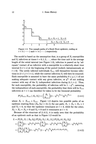
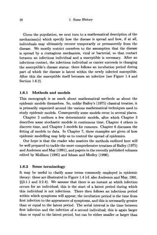
In the 20 years 1629-36 and 1647-58, there were 229 250 deaths recorded
from 81 different causes. Table 1.1 consolidates these data into eight main
groups. The relative risks of death from each of the eight causes are indi-
cated in the column furthest to the right in Table 1.1.
The main killers were Groups 1, 2 and 3; Graunt was led to observe that
whereas many persons live in great fear, and apprehension of some
of the more formidable, and notorious diseases following [Group 6]; I
shall onely [sic] set down how many died of each: that the respective
numbers, being compared with the Total of 229,250, those persons may
the better understand the hazards they are in.
The notorious diseases were further broken up by Graunt into the sub-
categories of Table 1.2. Among these, apoplexy appears to have been the
largest killer. Graunt's analysis of the various causes of death provided the
first systematic method for estimating the comparative risks of dying from
the plague, as against the chronical or other diseases, for example.
These observations may well be considered to be the first approach to
the theory of competing risks, a theory that is now well established among
modern epidemiologists.
1.2 A deterministic model
A more theoretical approach to the effects of a disease, namely smallpox,
was taken by Daniel Bernoulli (b. 1700, d. 1782) almost a century later.
Smallpox was then widespread in many parts of Europe where it affected

15. 1.2. A deterministic model
Table 1.2. Deaths due to notorious diseases
Causes
1. Apoplex
2. Cut of the stone
3. Falling sickness
4. Dead in the streets
5. Gowt
6. Head-ach
7. Jaundice
8. Lethargy
9. Leprosy
10. Lunatique
11. Overlaid, and starved
12. Palsy
13. Rupture
14. Stone and strangury
15. Sciatica
16. Sodainly
Total
Deaths
1306
38
74
243
134
51
998
67
6
155
529
423
201
863
5
454
5547
Risk xlO~3
5.697
0.166
0.323
1.060
0.585
0.222
4.353
0.292
0.026
0.676
2.308
1.845
0.877
3.764
0.022
1.980
24.196
Source: Graunt (1662).
a large proportion of the population, being responsible for around 10% of
the mortality of minors (cf. Bernoulli's model-based estimate in the last
column of Table 1.3) while those who survived were immune to further
attack but left scarred for life. In 1760 Bernoulli read his paper 'Essai
d'une nouvelle analyse de la mortalite causee par la petite verole et des
avantages de l'inoculation pour la prevenir' to the French Royal Academy
of Sciences in Paris. His intention was to demonstrate that variolation, i.e.
inoculation with live virus obtained directly from a patient with a mild case
of smallpox, a procedure that usually conferred immunity, would reduce the
death rate and increase the population of France. Bernoulli's argument is
readily recognized as the following problem in competing risks.
Suppose first that a cohort of individuals born in a particular year has
an age-specific per capita death rate ji{t) at age t. Then given an initial
population size £(0) = £0> its size £(£) at age t satisfies the equation
so
where M(i) is the cumulative hazard. We shall use £(•) below.
Consider another cohort subject to both the general per capita death
rate /x(t) as above and a further hazard (infection) like smallpox with a
constant infection rate (3 per individual per unit time. Individuals succumb
= £(0) exp ( - ft n(u) du) = £(0)e~M
«) = C(t), (1.2.2)

16. 1. Some History
Table 1.3. Age profile of population afflicted with smallpox (Bernoulli)
Age (yrs)
t
0
1
2
3
4
5
6
7
8
9
10
11
12
13
14
15
16
17
18
19
20
21
22
23
24
Total
&(*)
1,300
1,000
855
798
760
732
710
692
680
670
661
653
646
640
634
628
622
616
610
604
598
592
586
579
572
Age cohort
Immune
z(t)
0
104
170
227
275
316
351
381
408
433
453
471
486
500
511
520
528
533
538
541
542
543
543
542
540
Suscept.
x(t)
1,300
896
685
571
485
416
359
311
272
237
208
182
160
140
123
108
94
83
72
63
56
48.5
42.5
37
32.4
Smallpox
Incidence
137
99
78
66
56
48
42
36
32
28
24.4
21.4
18.7
16.6
14.4
12.6
11.0
9.7
8.4
7.4
6.5
5.6
5.0
4.4
Cumulative
Deaths
17.1
29.5
39.2
47.5
54.5
60.5
65.7
70.2
74.2
77.7
80.7
83.4
85.7
87.8
89.6
91.2
92.6
93.8
94.8
95.7
96.5
97.2
97.8
98.3
Annual
Total
300
145
57
38
28
22
18
12
10
9
8
7
6
6
6
6
6
6
6
6
6
6
7
7
Mortality
Smallpox
17.1
12.4
9.7
8.3
7.0
6.0
5.2
4.5
4.0
3.5
3.0
2.7
2.3
2.1
1.8
1.6
1.4
1.2
1.0
0.9
0.8
0.7
0.6
0.5
Source: Bernoulli (1760). Note that Halley's table (column 1) starts at t = 1; Bernoulli
gives reasons for choosing cohort size 1,300 for t = 0. Bernoulli used a = ft = 1/8, and
obtained his figures by smoothing to the mid-point of the previous year, so his figure 17.1
for t = l , coming from 1017.1, differs from 1014.9 = 8x 1000/[7 + exp(-l/8)] as follows
from (1.2.6) (cf. Gani, 1978).
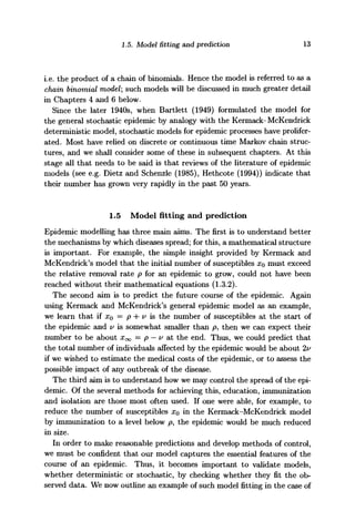
only once, the result of such infection being either death in a fraction a of
cases or immunity for the remainder of life in the complementary fraction
I — a. Denote the number of individuals still susceptible to the disease
at age t by x(t), and the total number of the surviving cohort of age t,
whether immune or not, by £p(t) as shown in Figure 1.1. To simplify the
mathematical model, the infectious state is assumed to be instantaneous,
so that as soon as an infection occurs, the infective individual either dies or
recovers immediately. Then for the x(t) susceptibles and z(t) = £@{t) —x(t)
immunes in this cohort,
x(t) =-(n(t) + 0)x(t) (1.2.3a)
and
z(t) = -v{t)z{t) + (1 - a)/3x(t). (1.2.3b)

17. Cohort
size
1200-
1000-
800-
6 0 0 -
4 0 0 -
200-
0
0
1.2. A deterministic model
10
I
15
I
20
-+- Age (years)
Figure 1.1. Survivors £/? ( ) and immunes z ( ) in cohort of
initial size 1300 (data from Table 1.3). The susceptibles of age t in the
cohort are x(t) = £#(£) — z(t).
These equations are solved via integrating factors. Using M(t) and x(0)
£(0) = £(0) = £0 a s
before, we have
whence
and
x(t) =
Integrating on (0, t) and simplifying,
(1.2.4)
- e""')
(1.2.5)
using (1.2.2); observe that £(£) = £0(£) when the infection rate (3 = 0.
Equation (1.2.5) relates the sizes of the surviving cohorts of age t in pop-
ulations with ({3 > 0) and without (/? = 0) smallpox, respectively. Bernoulli
used it in the form
(1.2.6)
1 - a + ae-#
to estimate the size of a surviving cohort £(£) in a 'state without smallpox'
on the basis of Halley's (1693) data from Breslau, now Wroclaw. This esti-
mation required parameters a and /?; on reviewing what evidence he could

18. 1. Some History
from a number of areas, Bernoulli fixed on a = j3 = 0.125. Use of these
estimates in (1.2.6) yields the data in the last column of Table 1.3; entries
in the other columns are derived from this column and Halley's data. Ob-
serve that, granted the validity of Bernoulli's assumptions, smallpox caused
between 10 and 40% of deaths between ages 2 and 23.
Suppose Bernoulli had had available observations of the form of his £(•)
at (1.2.6), for a 'state without smallpox' with a death rate similar to that
/JL(-) prevailing in the areas from which Halley's data were drawn (column 2
of Table 1.3). Then taking differences of (1.2.5) with itself for times t = t'
and t = t' 4- 1 yields
so that
In A(fr(f)/C(O) = "(<» + 0 0 , (1-2-7)
where a = — ln[a(l — e~^)]. This is the simplest way of expressing the
result (1.2.5) for the purpose of estimating f3 and a conditional on such
extended data being available. All that Bernoulli could do was to present
the advantage of variolation (i.e. absence of deaths due to smallpox) on the
basis of his model-based calculations. Note too that the population risk
of death from smallpox (cf. Tables 1.1-2) as implied by Table 1.1 is about
100/1300 « 7.7%, higher than in Table 1.1 because the London population
from which Graunt drew his data, included more immigrants than Breslau.
In Halley's day Breslau had rather few immigrants, and hence, propor-
tionately more infant and childhood deaths, smallpox being more prevalent
amongst children than adults.
1.2.1 The Law of Mass Action
The Law of Mass Action has found wide applicability in many areas of
science. In chemistry, the idea that a reaction is influenced by the quantities
of the reactant materials goes back at least to Boyle (c. 1674). Around 1800,
C. L. Berthollet emphasized the importance of mass or concentration of a
substance on a chemical reaction, but this was not generally accepted for half
a century. Ultimately, Guldberg and Waage (1864-1867) postulated that
for a homogeneous system, the rate of a chemical reaction is proportional
to the active masses of the reacting substances (Glasstone (1948, p. 816)).
Applied to population processes, if the individuals in a population mix
homogeneously, the rate of interaction between two different subsets of the

19. 1.3. From curve-fitting to homogeneous mixing models
population is proportional to the product of the numbers in each of the
subsets concerned. In any population it is possible for several processes to
occur concurrently, in which case the effects on the numbers in any given
subset of the population from these various processes are assumed to be
additive. Thus, in the case of epidemic modelling, the Law is applied to
rates of transition of individuals between two interacting categories of the
population, such as susceptibles who, as a result of contact with infectives,
themselves become infectives; a second simultaneous process is that of the
infectives who become removals. These two processes underlie equations
(1.3.2a) and (1.3.2c) respectively: when more than one process is involved,
as for the numbers of infectives in equation (1.3.2b), the effects are additive.
Application of the Law to transitions that occur in discrete time is not so
straightforward, but, subject to certain constraints on the size of the change
involved (see e.g. Section 2.8 below), it remains valid.
The Law also has a stochastic version when the process concerned is as-
sumed to be Markovian, and the rate is then interpreted as the infinitesimal
transition probability.
Implicit in the 'proportionality' aspect of the Law, is an assumption that
the quantities concerned in inducing the transition are subject to homoge-
neous mixing with each other. The Law can then be seen as the result of
superposing all possible contributions of the individual components to the
interaction, these individuals being regarded as equally likely to interact
with each other in a given (small) interval of time.
1.3 From curve-fitting to homogeneous mixing models
First issued in 1837, each Annual Report of the Registrar-General ofBirthsy
Deaths and Marriages in England included tables of causes of death and
commentaries. The Report for 1840 includes a contribution from William
Farr1
entitled 'Progress of epidemics', in which Farr attempted to char-
acterize mathematically the smoothed quarterly data for smallpox deaths.
Some 26 years later, in a letter to the London Daily News of 17 February
x
Farr was appointed compiler of abstracts to the General Register Office in 1839 and
remained there until retirement in 1879. Early volumes of the Annual Reports contain
papers of Farr prefaced by a 'Letter to the Registrar-General'; they cover a variety of
issues pertaining to the data in the Reports. Thus, in the Sixth Annual Report (1842)
Farr noted that the annual small-pox death-rates per 106
live individuals for the years
1838-42 were 1101, 604, 679, 408 and 172 respectively, and remarked that 'The reduction
in the mortality from small-pox since 1840 was probably the result, at least in part, of
the Vaccination Act' [of 1840]. Later he gave the 1850 death-rate as 263.

20. 1. Some History
Table 1.4. Deaths from smallpox in consecutive quarters 1837-39
Observed deaths
Deaths averaged over
two consecutive quarters
Percentage change
Sum.
1837
2513
Aut.
1837
3289
Win.
1838
4242
Spr.
1838
4484
Sum.
1838
3685
Aut.
1838
3851
Win.
1839
2982
Spr.
1839
2505
Sum.
1839
1533
Aut.
1839
1730
2901 3766 4365 4087 3767 3416 2743 2019 1637
+30 +16 -6 -8 -9 -20 -26 -19
Source: Farr (1840).
1866 (quoted by Brownlee, 1915), he attempted to predict the spread of
rinderpest among cattle by a similar method.
Table 1.4 gives the observed deaths in the smallpox epidemic of 1837
39 drawn from Farr (1840), together with the average values of consecutive
quarters, for 10 quarters in all. Farr concluded that as the epidemic declined,
he could detect an approximately steady rate of deceleration in the number
of deaths per quarter. Brownlee (1906) later carried out work of a similar
type: he fitted Pearson curves to epidemic data for several diseases, and for
several different locations.
But these pragmatic approaches were essentially limited, so long as there
was not an appropriate theory to explain the mechanism by which epidemics
spread. By the beginning of the twentieth century, the idea of passing on
a bacterial disease through contact between susceptibles and infectives had
become familiar, and Hamer (1906) first foreshadowed the simple 'mass
action' principle for a deterministic epidemic model in discrete time. This
principle, which incorporates the principle of homogeneous mixing, has been
the basis of most subsequent developments in epidemic theory (see Section
1.2.1 above and Anderson and May (1991, p. 7) for discussion).
Hamer, noticing the rise and fall of infectives in the course of a large
range of epidemics, argued against variable infectivity. Specifically, he wrote
that to explain the eventual decline of an epidemic, 'the assumption of
loss of virulence or infecting power on the part of the organism is quite
unnecessary'. He also put forward a numerical argument about the initial
increase and eventual decline of the number of infectives in a population; this
indicates that he was aware that both susceptibles and infectives affected the
number of new infectives listed in the weekly reports of measles in London:
Now the outbreak will take much longer to decline to extinction than it
took to rise, for those especially exposed have in large part been already
attacked and the disease must spread, in the main, among persons
whose manner of life brings them comparatively little into contact with
their fellows.

21. 1.3. From curve-fitting to homogeneous mixing models
Let xt, yt be the numbers of susceptibles and infectives respectively at
times t = 0,1,2,... . Hamer's idea was equivalent to expressing the new
number of infectives at time t 4- 1 by Ayt such that
Ayt=Pxtyt (4 = 0,1,2,...) (1.3.1)
where the constant (3 is such that (3xtyt < xt for all t, i.e. (3 < l/(maxi>i yi).
These new infectives are a proportion (3 of the number xtyt of contacts be-
tween susceptibles and infectives, where /? is known as the infection param-
eter. Because of the constraint on /?, it follows that in a closed population
in which yt — N — xu we have (3xt(N — xt) < xt or f3(N - xt) < 1; this is
certainly satisfied if /3 < 1/N.
Continuous time versions of epidemic equations were used by Ross (1916)
and Ross and Hudson (1917) in their studies of populations subject to in-
fection. But the form of equations most commonly used to characterize the
typical general epidemic with susceptibles x(t), infectives y(t) and immunes
z(t) (such as a measles epidemic) is due to Kermack and McKendrick (1927).
They assumed a fixed population size N = x(t) H- y(t) 4- z(t), and using the
homogeneous mixing principle for continuous time t > 0 derived the (now)
classical equations
d^c
-77 = -0xy, (1.3.2a)
d£
^ = 0xy - 7i/, (1.3.2b)
^ = 72/, (l-3.2c)
subject to the initial conditions (x(0),2/(0),z(0)) = (xo,2/o>0)- Here (3 is2
the infection parameter, similar to that in (1.3.1), and 7 is the removal
parameter giving the rate at which infectives become immune. In cases
where death or isolation may occur, z(t) represents all removals from the
population, including immunes, deaths and isolates.
Dividing equation (1.3.2a) by (1.3.2c) gives
dx (3 x , 7
— = x — with P=~3>
dz 7 p (3
the parameter p being the relative removal rate. The solution of this equa-
tion is
x = xoz-z/p
,
2
Some authors write (3 = (3'/x(0) so (1.3.2a) becomes x = -0'(x/xo)y.

22. 10 1. Some History
w=N-z
0 2oo
(a) XQ < p (b) xo > p
Figure 1.2. z^ as the point of intersection of w = N — z and w = xo e"
so that
Hence
with the parametric solution
= N-z- xoe~z/p
.
•/o
(0<t< oo). (1.3.3)
Kermack and McKendrick obtained two basic results, referred to as their
Threshold Theorem. The first is a criticality statement, and comes from
equation (1.3.2b). Writing this equation as
shows that if the epidemic is ever to grow, then we must have dy/dtt_0 > 0,
or xo > p, i.e. the initial number of susceptibles must exceed a threshold
value p. The second, deduced from (1.3.3), states that as t —> oo, z(i) —>
Zoo < N. Now in the limit t —• oo, N — z^ — x0e~ZoG
^p
= 0 (see the graphs
in Figure 1.2).
Suppose now that x0 is close to N; then z^ will be the approximate
solution of
0 = N - Zoo - N -
- f +
p > <»*•>

23. 1.4. Stochastic modelling 11
so that if N = p -- v with i / « p , then
Zoo ~ T ^ T - ~ 21/. (1.3.5)
1 + I//P
Thus, if x0 « A/" = p -f i/ with */ > 0, then since 2/oo = 0, Xoo + ^oo = A/" gives
(see Exercise 1.1 for the next term in the approximation).
Kermack and McKendrick's paper also includes the observation that, ac-
cording to the model, some susceptibles survive the epidemic free from in-
fection. At the time this was a significant result. We may view these three
results, stated formally later at Theorem 2.1, as typical of the qualitative
insights which mathematical models of epidemics attempt to achieve.
1.4 Stochastic modelling
The spread of an infectious disease is a random process; in a small group of
individuals, one of whom has a cold, some will catch the infection while oth-
ers will not. When the number of individuals is very large, it is customary to
represent the infection process deterministically as, for example, Anderson
and May (1991) mostly do. However, deterministic models are unsuitable
for small populations, while in larger populations, the mean number of in-
fectives in a stochastic model may not always be approximated satisfactorily
by the equivalent deterministic model.
One of the earliest of stochastic models is due to McKendrick (1926),
but the most used may well be the chain binomial model of Reed and
Frost, put forward in their class lectures3
at Johns Hopkins University in
1928, and based on one originally suggested by Soper (1929). Reed and
Frost never published their work; Helen Abbey (1952) later gave a detailed
account of it (see also Wilson and Burke (1942, 1943)). It should however be
pointed out that En'ko (1889) anticipated some aspects of Reed and Frost's
model by nearly 40 years, fitting data on measles epidemics recorded in
St. Petersburg to a discrete time model similar to theirs (see En'ko (1889)
and Dietz (1988)).
3
E. B. Wilson records these dates as February 2-3, 1928, and refers to correspondence
with Dr Frost shortly thereafter: 'I strongly urged Dr Frost to publish his theory of the
epidemic curve, but he thought it too slight a contribution' (Wilson and Burke, 1942,
note 3).

24. 12 1. Some History
xt
5
4
3
2
1 : = X3 = 1, ^3=0
JT3 = X4 = 0, = 0
0 1 2 3 4
Figure 1.3. Two sample paths of a Reed-Frost epidemic, ending at
t = 3 ( ) and £ = 4 ( ) respectively.
The model is based on the assumption that, in a group of Xt susceptibles
and Yt infectives at times t = 0,1,2,..., where the time unit is the average
length of the serial interval (see Figure 1.3), infection is passed on by 'ad-
equate' contact of an infective with a susceptible in a relatively short time
interval (£, t + t) at the beginning of the period (indeed, instantaneously at
t + 0). The newly infected individuals Yt+ will themselves become infec-
tious in (£ + 1, £-hl-he), while the current infectives Yt will then be removed.
Each susceptible is assumed to have the same probability 0 < q < 1 of not
making adequate contact with any given infective, or qYt
of not making
contact with any of the Yt independent infectives during (£, t -h e). Thus,
for each susceptible, the probability of infection will be 1 — qYt
; assuming
the independence of each susceptible, the probability that there will be Yt+
infectives at t + 1 can therefore be taken to be the binomial probability
Xt
Xt,Yt} = (1.4.1)
where Xt = Xt+ + lt+i. Figure 1.3 depicts two possible paths of an
epidemic starting from (Xo, Yo) = (4,1); for one path, X > X2 = X3 = 1
and y3 = 0, so that the epidemic terminates at t = 3, while for the other,
X2 > X3 = Xt = 0 and Y4 = 0 and it terminates at t = 4.
Because of the structure of (1.4.1), it is easily seen that the probability
of an epidemic such as that in Figure 1.3 would be
L = P{XuY1X0,Y0}P{X2,Y2X1,Yl}P{X2,0X2,Y2}
x2
(1.4.2)

25. 1.5. Model fitting and prediction 13
i.e. the product of a chain of binomials. Hence the model is referred to as a
chain binomial model; such models will be discussed in much greater detail
in Chapters 4 and 6 below.
Since the later 1940s, when Bartlett (1949) formulated the model for
the general stochastic epidemic by analogy with the Kermack-McKendrick
deterministic model, stochastic models for epidemic processes have prolifer-
ated. Most have relied on discrete or continuous time Markov chain struc-
tures, and we shall consider some of these in subsequent chapters. At this
stage all that needs to be said is that reviews of the literature of epidemic
models (see e.g. Dietz and Schenzle (1985), Hethcote (1994)) indicate that
their number has grown very rapidly in the past 50 years.
1.5 Model fitting and prediction
Epidemic modelling has three main aims. The first is to understand better
the mechanisms by which diseases spread; for this, a mathematical structure
is important. For example, the simple insight provided by Kermack and
McKendrick's model that the initial number of susceptibles XQ must exceed
the relative removal rate p for an epidemic to grow, could not have been
reached without their mathematical equations (1.3.2).
The second aim is to predict the future course of the epidemic. Again
using Kermack and McKendrick's general epidemic model as an example,
we learn that if xQ = p + v is the number of susceptibles at the start of
the epidemic and v is somewhat smaller than p, then we can expect their
number to be about Xoo = p — v at the end. Thus, we could predict that
the total number of individuals affected by the epidemic would be about 2v
if we wished to estimate the medical costs of the epidemic, or to assess the
possible impact of any outbreak of the disease.
The third aim is to understand how we may control the spread of the epi-
demic. Of the several methods for achieving this, education, immunization
and isolation are those most often used. If one were able, for example, to
reduce the number of susceptibles XQ in the Kermack-McKendrick model
by immunization to a level below p, the epidemic would be much reduced
in size.
In order to make reasonable predictions and develop methods of control,
we must be confident that our model captures the essential features of the
course of an epidemic. Thus, it becomes important to validate models,
whether deterministic or stochastic, by checking whether they fit the ob-
served data. We now outline an example of such model fitting in the case of

26. 14 1. Some History
Table 1.5. The Ay cock measles epidemic
t
xt
Yt
0
111
1
1
108
9
2
86
22
3
25
61
4
12
13
5
12
0
Source: Abbey (1952).
a measles epidemic. If the model is validated, it can then be used to predict
the course of the epidemic in time.
Following the pioneering study of measles and scarlet fever by Wilson et
al. (1939), Abbey (1952) was among the first to use a stochastic epidemic
model for the estimation of a 'contact' parameter, and for testing the validity
of the model. Among her many sets of data was one for a particular measles
epidemic in 1934 studied by Aycock (1942); to this data set she decided to
fit a Reed-Frost model for t = 0,1,..., 5, the unit of time being a 12-day
period. Using the same notation as in the previous section, Table 1.5 records
the progress of the Aycock epidemic.
From the Reed-Frost model, the probabilities of these results in each
individual time interval can be worked out respectively as
__ ^922/^986
(1.5.1)
Abbey obtained estimates of the probabilities qi of no contact in each sep-
arate interval i = 1,2,3,4 by the Maximum Likelihood method as
=0.9454, fc=(_) =0.988.
If one assumes that the probability of no contact has the same value q
throughout all intervals, then the probability of the epidemic is given by
L(q) = Li(q)L2(q)L^(q)L/i(q)1 (1.5.3)
with functions Li as in (1.5.1). The Maximum Likelihood estimator q of q
satisfies the relation
dlnL 9 198<f 1342o21
793<f° 2320
= - 1 ~ ~ i ^ ~ i Too - -,—"W + —^- = °> (1-5.4)
q=q 1 - 9 1 - r l-q22
1-q61
q
dq
which can be solved numerically to yield q = 0.9685.

27. 1.6. Some general observations and summary 15
The fit of this model to the data turns out to be far from perfect: on a
goodness-of-fit test Abbey reported %2
= 53.1 on 4 degrees of freedom, and
noted a significantly improved fit from estimating (rather than counting)
the number of susceptibles. Abbey (1952) found the same true of other
measles, cHickenpox and German measles data, and investigated variation
of the contact rate either with time or between individuals, or both, as
other possible reasons for the inadequate fit of the model to the data (see
Chapter 4).
1.6 Some general observations and summary
Mathematical techniques and models used in the study of epidemics form
a major part of this book. They usually encompass, for any given model, a
set of assumptions which can roughly be described as belonging one to each
of the categories listed below.
The 'epidemic process' can be characterized as the evolution of some
infectious disease phenomenon within a given population of individuals.
The properties of the process fall naturally into three categories:
(1) assumptions about the population of individuals within which the dis-
ease first manifests itself, and then spreads;
(2) assumptions about the disease mechanism: how it is spread, and the
mechanism of recovery or removal, if such occurs; and
(3) mathematical modelling assumptions that allow the specification of the
two preceding properties.
So far as the population is concerned, we make assumptions about
(a) its general structure: it may be a single homogeneous group of individu-
als (apart from (c) below), or a collection of several homogeneous strata
or subgroups, or else generally heterogeneous so that each individual is
different;
(b) the population dynamics which specify whether the population is closed
so that it is a constant collection of the same set of individuals for
all time, or open, allowing individuals to give birth and die, and to
emigrate or immigrate or both; and
(c) a mutually exclusive and exhaustive classification of individuals ac-
cording to their disease status-, thus, at any given time, an individual is
either susceptible to the disease, or incubating it, or infectious with it,
or possibly an infectious carrier without any symptoms of the disease,
or a 'removed case.' A removal has been infectious or an infectious
carrier but is so no longer, whether by acquired immunity or isolation
or death.

28. 16 1. Some History
Given the population, we next turn to a mathematical description of the
mechanism(s) which specify how the disease is spread and how, if at all,
individuals may ultimately recover temporarily or permanently from the
disease. We mostly restrict ourselves to the assumption that the disease
is spread by a contagious mechanism, viral or bacterial, so that contact
between an infectious individual and a susceptible is necessary. After an
infectious contact, the infectious individual or carrier succeeds in changing
the susceptible's disease status: there follows an incubation period during
part of which the disease is latent within the newly infected susceptible.
After this the susceptible itself becomes an infective (see Figure 1.4 and
Section 1.6.2).
1.6.1 Methods and models
This monograph is as much about mathematical methods as about the
epidemic models themselves. So, unlike Bailey's (1975) classical treatise, it
is primarily organized around the various mathematical techniques used to
study epidemic models. Consequently some models recur in several places.
Chapter 2 outlines a few deterministic models, after which Chapter 3
describes some stochastic models in continuous time, Chapter 4 others in
discrete time, and Chapter 5 models for rumours. Chapter 6 discusses the
fitting of models to data. In Chapter 7, three examples are given of how
epidemic modelling may help us to control the spread of epidemics.
Our hope is that the reader who masters the methods outlined here will
be well prepared to tackle the more comprehensive treatises of Bailey (1975)
and Anderson and May (1991), and papers in the recently published volumes
edited by Mollison (1995) and Isham and Medley (1996).
1.6.2 Some terminology
It may be useful to clarify some terms commonly employed in epidemic
theory: these are illustrated in Figure 1.4 (cf. also Anderson and May, 1991,
§§3.1.1 and 3.2.4). We assume that there is an instant at which infection
occurs for an individual; this is the start of a latent period during which
this individual is not infectious. There then follows an infectious period
within which symptoms will appear; the incubation period is the time from
first infection to the appearance of symptoms, and this is necessarily greater
than or equal to the latent period. The serial interval is the time between
first infection and the infection of a second individual; this is again larger
than or equal to the latent period, but can be either smaller or larger than

29. 1.7. Exercises and Complements to Chapter 1 17
Individual's
disease state: Susceptible Latent < Infectious > Immune/Removed
1 1 1 1 1 > time
Epoch: tA tB tc t£> tE
<— Incubation period —>
< Serial interval •
tj'. Infection occurs £#: Latency to infectious transition
tc- Symptoms appear t^: First transmission to another susceptible
tE- Individual no longer infectious to susceptibles (recovery or removal)
Note: tp is constrained to lie in the interval (iB»^i?)» s o
t& > tc (as shown) and
tD < tc are both possible.
Figure 1.4. Diagrammatic representation of progress of a disease in an
individual.
the incubation period. Often the serial interval and latent period are used
interchangeably although their meanings are different. The fundamental
quantity in the process of infection is the serial interval, but the latent period
is often used in the literature because it is assumed that a second infection
will occur as soon as the first infective becomes infectious. Anderson and
May (1991, §3.2.4) use the term generation time of the disease agent; in
terms of the notation in Figure 1.4 it is the expectation of (£# — t^) +
(tE — £#)> i-e. the mean latent period plus half the mean infectious period.
1.7 Exercises and Complements to Chapter 1
1.1 Show that for positive n, e and p there exists a unique root of the equation
n +e = z + ne~z/p
satisfying 0 < z — e < n, z = (, say. Expand the exponential term to third
order and deduce that in the limit e [ 0, Q « 2v — v2
1 p where 0 < v =
n - p = O(pi) (cf. Daley and Gani, 1994, §4.1). (The notation here and of
equation (1.3.4) is related by z = Zoo, n = xo and n + e = N.)
1.2 In the general epidemic model sketched in Section 1.3, the quantity Ro =
n/p = /3n/j = (initial no. of susceptibles)/(relative removal rate) coincides
with the Basic Reproduction Ratio in Section 3.5 below. Show that for
Ro = 2 in this model starting from t/o < ^o, about 20% of the population
survive the epidemic. Bartholomew (1973, p. 346) gives 2% for Ro — 4.
1.3 The data in Table 1.6 come from bar charts labelled a, ..., j in En'ko (transl.
1989). En'ko extracted the daily numbers of measles cases for several years
from records at the St Petersburg Alexander Institute, where the date of a
measles case was determined by the appearance of a rash on the face, and
at the Educational College for the Daughters of the Nobility, where the date
was determined by the date of transfer into the infirmary. En'ko allocated
cases recorded 0-7, 8-17, 18-29, 30-41, 42-53, 54-65, ... days following the

30. 18 1. Some History
Table 1.6. Numbers of cases in successive generations ofseveral measles epidemics
1st
day
0
9
20
32
44
0
8
21
0
9
19
37
0
11
25
35
0
12
24
37
0
1
1
6
1
2
1
5
3
2
3
1
1
1
2
1
1
1
1
1
1
1 2 3
1865,
2
5
4
0
2
3
2
0
1875,
0
0
2
2
1879,
5
1
6
3
1882,
0
0
6
0
3
1
1884,
1
0
0
1
0
0
b
4
4
2
1
i
3
0
c
5
0
e
0
3
1
f
0
0
0
4
4
3
0
0
2
1
0
2
1
3
1
1
3
0
5
0
3
1
5
2
1
0
1
0
6
3
2
2
1
1
1
1
7
0
1
2
0
0
8 9
1
1
0 1
1
1
1st
day
0
10
22
34
46
0
9
19
35
0
8
18
32
0
11
20
29
51
0
8
19
31
44
60
69
85
0
1
2
2
2
4
1
1
1
1
2
2
2
1
1
1
2
3
1
13
7
5
2
4
1
1
1
1
1
4
0
3
2
22
5
0
1
5
3
0
1
1
2
0
0
2
1
3
18
11
1
1
4
1
1
0
3
0
0
1
4
4
7
4
4
7
0
1
1
4 5
1870, h
0
0
2
3
2
2
2
1
4
1
1874,g
12
3
7
5
1875,a
20
6
7
2
1888, d
1
2
0
Combined counts
2
10
18
3
0
0
34
21
7
5
0
43
18
4
3
0
39
18
8
4
1
1
1
6
1
0
4
0
17
5
5
0
2
0
7
1
0
1
1
6
5
1
1
1
8
2
1
1
1
2
0
2
> of 10 epidemics
2
25
17
6
4
0
18
12
13
3
1
13
18
6
1
6
10
7
0
9
0
2
1
2
2
. J
2
13
5
1
10
1
1
1
0
1
1
3
2
1
11
1
1
2
2
Source: From bar charts in En'ko (transl. 1989). See Exercise 1.3 for more explanation.
initial case on day 0, to generation 0, 1, ... respectively. The table gives for
each epidemic the first day of observing a case for each generation, and the
number of cases reported on the various days within the generation, for as
long as there were any such cases.
(a) Investigate whether the spread of the dates of recording cases within an
epidemic shows any systematic trend from one generation to another (if not,
then periodicity is strong, and identifying a case is variable).
(b) Repeat the analysis of (a) on the combined data: what sort of additional
variability does such pooling of data introduce?
(c) The construction of analogues of qt and q as in section 1.5 entails the
estimation of the population size as well.
(d) If a model is fitted as in (c), then a 2
goodness of fit test can be
performed.

31. 1.7. Exercises and Complements to Chapter 1 19
1.4 Wilson and Burke (1943) list the monthly numbers of measles cases in Prov-
idence RI for the years 1917-1940 as in Table 1.7. Plot out the course of the
nine epidemics for which the epidemic curves peak around May 1918, Mar.
1921, Mar. 1923, Jan. 1926, Apr. 1928, Jan. 1932, May 1935, Mar. 1937,
Mar. 1940. Observe that there is a marked seasonality effect if the dataset
is treated as a whole.
(a) Assuming a mean serial interval of 0.5 months and a closed population
for the course of the epidemic, investigate how estimates of any or all of JV,
/o, /3, 7 might be constructed.
(b) Repeat this analysis for the record as a whole assuming instead an
immigration of 2130 new susceptibles each September (thus, Aryear varies as
each year changes).
(c) Repeat the analysis of (b) but assuming now a steady immigration of
178 new susceptibles per month.
Table 1.7. Measles cases by months in Providence RI 1917-1940
Year
1917
1918
1919
1920
1921
1922
1923
1924
1925
1926
1927
1928
1929
1930
1931
1932
1933
1934
1935
1936
1937
1938
1939
1940
Total
Jan.
33
55
1
125
329
89
680
5
13
2057
5
45
84
2
1
2799
0
4
13
119
422
2
33
569
7485
Feb.
47
98
4
127
585
4
1228
6
11
1360
2
112
189
0
2
2037
0
11
57
74
811
5
35
495
7300
Mar.
62
373
4
136
665
3
1470
3
6
648
1
422
261
1
49
574
0
21
343
92
1184
4
40
530
6890
Apr.
109
1232
4
279
390
26
687
11
15
348
1
1081
399
4
158
199
3
18
1351
76
711
2
118
462
7684
May
119
1299
5
404
266
25
383
16
18
196
2
883
276
23
456
81
3
29
1953
83
472
0
317
543
7852
June
36
780
4
288
99
22
117
30
30
105
2
800
111
46
358
11
6
106
1279
17
129
0
286
372
4934
July
13
261
3
146
28
23
29
15
58
48
6
508
38
22
179
2
5
44
241
11
31
0
157
121
1989
Aug.
7
23
3
38
10
19
6
2
50
8
2
77
4
8
99
0
2
25
17
4
4
3
64
20
495
Sep.
2
8
1
45
1
7
3
2
13
1
0
18
3
1
22
0
4
8
4
0
0
1
20
1
165
Oct.
1
6
2
53
2
16
10
1
81
0
9
36
2
0
191
0
0
5
1
0
2
0
89
0
507
Nov.
8
5
1
190
7
131
7
5
417
0
7
36
0
2
337
0
1
1
0
9
3
0
267
1
1435
Dec.
55
3
3
191
26
652
7
2
1224
4
23
61
0
0
1548
0
1
7
48
77
3
3
446
1
4385
Total
492
4143
35
2022
2408
1017
4627
98
1936
4775
60
4079
1367
109
3400
5703
25
279
5307
562
3772
20
1872
3113
51221
Source: Wilson and Burke (1943).

32. Deterministic Models
In deterministic models, population sizes of susceptibles, infectives and re-
movals are assumed to be functions of discrete time t = 0,1,2,... or dif-
ferentiable functions of continuous time t > 0. Such approximations to the
true, integer-valued numbers of individuals involved in an epidemic, allow
us to derive sets of difference or differential equations governing the process.
The evolution of this epidemic process is deterministic in the sense that no
randomness is allowed for; the system develops according to laws similar to
those for dynamical systems. It is usual to regard the results of a determin-
istic process as giving an approximation to the mean of a random process:
there are examples related to this in the next chapter (see equations (3.2.4)
and (3.3.6), and Exercises 3.1, 3.2, 3.5 and 3.11).
2.1 The simple epidemic in continuous time
A simple epidemic is one where the population consists only of susceptibles
and infectives; once a susceptible is infected, it becomes an infective and
remains in that state indefinitely. A simple epidemic may be thought of as
one where
(a) the disease is highly infectious but not serious, so that infectives remain
in contact with the susceptibles for all time t > 0;
(b) the infectives continue to spread their infection until the end of the
epidemic (see equation (2.1.2) and below for interpretations of the 'end'
of the epidemic).
An infection which may approximate these conditions is the common cold
over a period of a few days. This simple epidemic model is the same as the
logistic model of population growth, attributed1
to Verhulst (1838).
1
Miner (1933) remarks that 'Verhulst's work was generally forgotten until after the
20

33. 2.1. The simple epidemic in continuous time 21
We suppose that the total population is closed, i.e.
x(t) 4- y(t) = N (all t > 0)
where, as throughout this chapter, x(t) and y(t) denote the numbers of
susceptibles and infectives at time t, with initial conditions (x(Q),y(0)) =
(%o-> Vo) with 7/o > 1. Then assuming that the individuals of the population
mix homogeneously, we can write
%=0xy = l3v(Ny), (2.1.1)
at
where /? is the pairwise rate of infection (i.e. infection parameter) and, in
contrast to the discrete time case (cf. (1.3.1)), the condition (3 < l/N is
no longer needed. This differential equation, the so-called logistic growth
equation, is readily solved, since
y(N-y) y N-yJ N
so integrating on (0, £),
l n ^ l n ^
N - y(t) N-y0
Hence
As t —> oo, equation (2.1.2) shows that y(t) —> N, so that according to the
model all individuals in the population eventually become infected, thus
causing the end of the epidemic (in the mathematical sense).
In this model we have both x(t) > 0 and y(t) > 0 for all finite positive
£, so the question arises as to when we may consider the epidemic to have
terminated in practical terms. Realistically, we could define the 'end' of the
epidemic to occur at Ti = inf{t : y(t) > N - 1}, i.e. when the number of
infectives is within 1 of its final value. Since the function y(-) has a positive
independent rediscovery of the logistic curve by Pearl and Reed in 1920', and that to his
knowledge 'the only reference to the work of Verhulst in modern times prior to [1920] is
[a paper in 1918 by Du Pasquier]'. Bailey (1975) gives no account of its emergence in
epidemic theory; Bailey (1955) attributes the stochastic version of the model to Bartlett's
1946 lecture notes (see Bartlett, 1947).

34. 22 2. Deterministic Models
derivative for finite t, T is determined by y(Ti) = N - 1. It follows from
(2.1.2) that
2/oiV __ KT 1
SO
Table 2.1 illustrates the values of T for various values of yo when N
24,50,100,1000 for the simple case where /? = I/AT.
Table 2.1. Ti determined from y{T) = N -1 when 0 = I/AT
2/0
1
10
N = 24
6.2710
3.3979
3.1355
50
7.7836
5.2781
3.8918
100
9.1902
6.7923
4.5951
1000
13.8135
11.5019
6.9068
Observe that as yo increases from 1 to |7V, the time T taken to reach
AT—1 is halved, as follows from the symmetry about y = ^N of the derivative
at (2.1.1). Also, as N increases from 24 to 1000, T increases rather slowly
for, as (2.1.3) shows, Tx = O((]nN)/0N).
Thus, if the unit of time is the day, in a classroom of 50 schoolchildren of
whom one has a cold initially, the infection spreads among the whole class
in fewer than eight days if (3N = O(l).
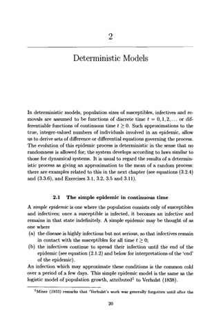
Sometimes epidemiologists are more interested in the epidemic curve,
which is the rate of occurrence of new infectives, here dy/dt. We see from
(2.1.1) that
dy _ pN2
y0(N - yo)e^Nt
_ (3yo(N - y0)
dt [yoePNt
+ (N - yo)}2
[cosh/3Nt + (l- 2yo/N) sinh 0Nt]2
'
(2.1.4)
It has a maximum when
At this time we have x(t) = y(t) = |JV, and (dy/dt) = /3(|JV)2
. The dashed
curve in Figure 2.1 illustrates equation (2.1.4), i.e. the epidemic curve for
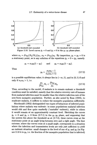
the deterministic model of a simple epidemic (cf. also Figure 2.12 below).

35. 2.2. The simple epidemic in interacting groups 23
y(t)
dy/dt
Figure 2.1. y(t) ( ) and dy/dt ( ) for the simple epidemic.
2.2 The simple epidemic in interacting groups
We suppose in this section that a closed population now consists of m groups
of sizes Ni,..., ATm, in each of which a simple epidemic may break out.
Assume that these groups interact with each other as follows. In place of
the single pairwise infection rate /? as in (2.1.1), suppose that susceptibles
in the j th group are subject to infection from infectives in the i th group at
rate fiij per interacting pair; for i = j we set /?j = jijj (j = 1,..., ra). Figure
2.2 illustrates the model, which is due to Rushton and Mautner (1955).
For ij = l,...,m:
Figure 2.2. Infection rates in interacting communities i,j = 1,... ,m.
Let Xj(t), yj(t) denote the numbers of susceptibles and infectives in each
of the groups j = 1,... ,m respectively. Then we readily see that when
infection is transmitted both within and between groups, equation (2.1.1)
can be generalized to the set of equations
dt + (j = 1,..., ra), (2.2.1)
subject to the initial conditions Vj(O) = yj0 and Xj(0) = Nj — yjO, as follows
from Xj = Nj — yj.

36. 24 2. Deterministic Models
While these equations may be solved numerically, explicit algebraic results
are obtainable only if the parameters and initial values have a relatively
simple structure. For example, we might set f3j = (3 (all j) and fyj = /3K for
some K ^ 1 for infection between different groups. Then (2.2.1) becomes
(2.2.2)
dt
A further simplification is to set Nj = N (all j). Then (2.2.2) becomes
(j = l,...,m). (2.2.3)
If all the initial values t/jo — Vo are the same, this set of equations basically
reduces to the single equation
- y)y[l + (m - l)/c] =
where /?' = /3[1 -j- (m — 1)K] and
VoN
as is consistent with (2.1.2) when m — 1.
We now show that if the yjo are different but N3 = N for all j , there
exist explicit parametric solutions of (2.2.3) for the yj(t). Write r = fit,
a = 1 -f (m — 1)K and Xj = N — yj. Then (2.2.3) becomes
— (j = l,...,m). (2.2.4)
The further transformations Uj = eaNT
(xj/N) and v = (1 - e~aNT
)/a lead
to
— lnLT,- = C^ + K (j = 1,... ,m), (2.2.5)
or in terms of m-vectors U and InU and the mxm matrix B = (6^) defined
by
I/2
lnU =
f lnC/i 1
lnC/2
Un(7mJ
' 1

37. 2.2. The simple epidemic in interacting groups 25
where In U involves an abuse of notation,
lnU BU. (2.2.6)
dv
Note that for t = 0, r = 0, v = 0 and xj0 = N - yj0 = NUj(0).
This matrix equation can be solved as follows. First use the inverse
B 1
= (bij
) of B (assuming |B| ^ 0) to give
dv
i.e.
d m
2 = 1
Define X by setting In X = B - 1
In U, so that In U = B In X. These relations
are equivalent to
from which it follows that
d
- In Xj = Uj=
i=l
Then for all j = 1,..., m,
V ^ = (flrf = F(v) say. (2.2.8)
i=l
Hence on integration,
X«-v) - X«-0) = (K - 1) T F(u) du = G(v),
Jo
or
r ] vc^-i) ii/(«-i)
F(ii)duj = [Xp^+Giv)]
where X,(0) = nili^fl
(0) = UZo (*Jo/Nf Now from (2.2.7), for all
j = l,...,m,

38. 26 2. Deterministic Models
But from (2.2.8),
,K/(,C-1)
K - 1 dv '
whence
v =
n. K. — 1 /o,
so that the time is given parametrically in terms of G. We can now find the
solutions for Uj(v) and hence for the original yj — N — Ne~aN
Pt
Uj.
These computations simplify as follows in the special case where yio — 1
and yjo — 0 for j = 2,..., ra, so the y3,(t) for j = 2,..., m are identical for
all t > 0, and equations (2.2.4) reduce to the two equations
Further transformations as in (2.2.5) lead to
= xi + (m — 1)«£2 — Na,
( 2
- 2
- n )
[1 + (m - 2)«]a;2 - iVa.
lnC/2 J - { K 1 + ( m - 2)K J I f/2 J - B
I C/2
We note that
! _ 1 (l + (m-2)K - ( m - l ) « l
- ^ I 1 JB
where
X = |B| = 1-f (m - 2)« - (m - 1)K2
= (1 - k)[l + (m
so that
It follows that when £ = 0, v = 0 and
Xt(0) = u[1+{m
-2)K]/K
(0)U^{m
~1)/K
(0) = (1 - # - i
X2(0) = UiK/K
(0)Ul/K
{0) = (1 - AT-1
)""7
^.

39. 2.3. The general epidemic in a homogeneous population 27
/
/
/
J
>']
1
/
fh
k
'
w
w
o t o
(a) K = 0.1
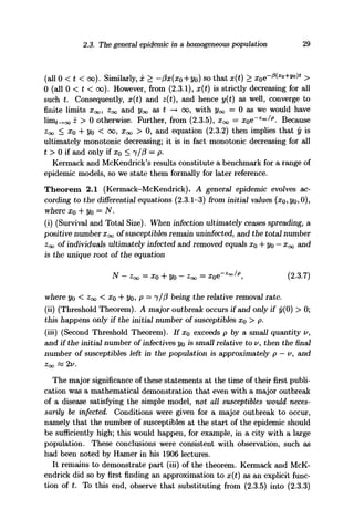
Figure 2.3. Numbers of infectives y and 2/2 (
and y2 ( ), for a Rushton-Mautner simple epidemic spreading in two
communities, with #i(0) = £2(0) = N, yi(0) = 1 and 2/2(0) = 0, and K as
shown.
(b) « =
), and infection rates y
Hence
Xi(v) = ((1
X2(v) - ((1
where
v = — 1
K
~ l
Jo
'd5 . (2.2.13)
Hence, for any time v, G(v) is known by (2.2.13), and thus also X{v) and
X2(v). Prom these Ux{v) and U2(v) are obtained as Ui = ^X^771
"1
^ and
C/2 = X ^ 1
" ^ ^ "2
^ , and thus z, and Vj = N - Xj (j = 1,2).
Figure 2.3 depicts the spread of infection in a population of two equally
sized strata. For larger K as in (a), the outbreaks largely overlap and re-
inforce each other, whereas in (b) the epidemics occur more slowly and
approximately in sequence.
2.3 The general epidemic in a homogeneous population
In the classical model for a general epidemic that we now describe, the size
of the population N is assumed to be fixed as for the simple epidemic of

40. 28 2. Deterministic Models
Section 2.1, but infectives may die, be isolated, or recover and become im-
mune. Individuals in the population are counted according to their disease
status, numbering x(t) susceptibles, y(t) infectives and z(t) removals (dead,
isolated or immune), so that x(t) is non-increasing, z(t) non-decreasing and
the sum x(t) + y(t) -b z(t) = JV, for all t > 0. The differential equation
governing x(t) is
d^c
— = -(3xy, (2.3.1)
where /? > 0 is the pairwise rate of infection as before, and (x,y, z)(0) =
(#o>2/o?2o) with yo > I, zo = 0. The number of infectives simultaneously
increases at the same rate as the number of susceptibles decreases, and
decreases through removal (by death, isolation or immunity) at a per capita
rate 7 > 0, so that
^ L i y . (2.3.2)
Finally the number of removals increases at exactly the same rate as the
loss of infectives, so that
ft=iv. (2.3.3)
Observe that (d/dt)(x(t) + y(t) + z(t)) = 0, as is consistent with the total
population size remaining fixed at TV.
In their first paper entitled 'A contribution to the mathematical theory of
epidemics', Kermack and McKendrick (1927) proposed these equations as
a simple model describing the course of an epidemic. We can write (2.3.1)
and (2.3.3) as
l . d * = _ 0 d z = _ l dz
x dt 7 dt p dt' K }
where p = 7//? is the relative removal rate. Integrating this differential
equation directly, and using the initial values xo and z0 — 0 as above, we
obtain
x(t) = zo e-2 ( t ) / p
. (2.3.5)
A second integral is also readily obtained: equations (2.3.1-2) imply that
x(t) and y(t) satisfy
ax x
so
x(t) + y(t) - plnx(t) =xo + yo- plnx0. (2.3.6)
Within the region where x, y and z are non-negative, equation (2.3.2)
yields the inequality y > -7?/, which in turn implies that y(t) > yoe~l1
> 0

41. 2.3. The general epidemic in a homogeneous population 29
(all 0 < t < oo). Similarly, x > -px(xo+yo) so that x(t) >
0 (all 0 < t < oo). However, from (2.3.1), x(t) is strictly decreasing for all
such t. Consequently, x(t) and z(t), and hence y(t) as well, converge to
finite limits XQO, Z^ and ^ as t -> oo, with y^ — 0 as we would have
lim^ooi > 0 otherwise. Further, from (2.3.5), XQO = x0e~Zoo/p
. Because
z<x> < #o + 2/o < oo, XQO > 0, and equation (2.3.2) then implies that y is
ultimately monotonic decreasing; it is in fact monotonic decreasing for all
t > 0 if and only if x0 < 7//? = p.
Kermack and McKendrick's results constitute a benchmark for a range of
epidemic models, so we state them formally for later reference.
Theorem 2.1 (Kermack-McKendrick). A general epidemic evolves ac-
cording to the differential equations (2.3.1-3) from initial values (xo,2/o?O),
where x0 + Vo = N.
(i) (Survival and Total Size). When infection ultimately ceases spreading, a
positive number XOQ of susceptibles remain uninfected, and the total number
Zoo of individuals ultimately infected and removed equals xo + yo — x<x> and
is the unique root of the equation
N-zoo = x0 + y0-zoo= xoe-Zo
°/p
, (2.3.7)
where yo < Zoo < #o + 2/o? P — i/P being the relative removal rate.
(ii) (Threshold Theorem). A major outbreak occurs if and only if y(0) > 0;
this happens only if the initial number of susceptibles Xo > p.
(iii) (Second Threshold Theorem). If XQ exceeds p by a small quantity u,
and if the initial number of infectives yo is small relative to v, then the final
number of susceptibles left in the population is approximately p — v, and
Zoo « 2V.
The major significance of these statements at the time of their first publi-
cation was a mathematical demonstration that even with a major outbreak
of a disease satisfying the simple model, not all susceptibles would neces-
sarily be infected. Conditions were given for a major outbreak to occur,
namely that the number of susceptibles at the start of the epidemic should
be sufficiently high; this would happen, for example, in a city with a large
population. These conclusions were consistent with observation, such as
had been noted by Hamer in his 1906 lectures.
It remains to demonstrate part (iii) of the theorem. Kermack and McK-
endrick did so by first finding an approximation to x(t) as an explicit func-
tion of t. To this end, observe that substituting from (2.3.5) into (2.3.3)

42. 30 2. Deterministic Models
together with the constraint on the population size yields
dz
i ^ . ~v
j •"u^ / • yZ.o.o)
This differential equation does not have an explicit solution for z in terms of
t. However, using the expansion e~u
= 1 — u + v? + O(u3
) and neglecting
the last term, yields the approximate relation
which can be solved. First express the right-hand side as in
2 x
° i f x
° A 2
fx
° 2
Now setting
a=JQ(N-xo)+(—--l (2.3.10)
this reduces to
dz p2
Substitute
atanh^^f.-pp2
L xo p
where at time t = 0, z0 = 0, so that atanht;0 = — [(#o/p) ~ !]• Then we
can readily see with this substitution in (2.3.11) that
Hence
d^ P2
J , 2 2 , U2 P2
u2 d v
-r « -— a - a tanh v) = —asech v—.
dt 2x0
v f
x0 dt
dv T ,
— « f7a, so v « ^7^ -h
and
i (£2 ) ^ ! tanh (I7erf - ^) (2.3.12)()
XQ
" 1
with </? = tanh"1
[(l/a)((xo /p) - l)].

43. 2.3. The general epidemic in a homogeneous population 31
Equation (2.3.12) yields an approximation to Zoo = lim^oo z(t),
namely
( Y (2-3.13)
Xo p
Now from equation (2.3.10) for a, when 2XQ(N — XQ) <<C (ZO — p)2
and
x0 > p,
(2.3.14)
or, writing XQ = p + ^ for some positive z/,
~
Equivalently, XQQ ~p--v — 2v = p — V. Note that this result is obtained
from the approximation (2.3.9) to the differential equation (2.3.8).
Another route to part (iii) of Theorem 2.1 is to analyse equation (2.3.5)
more directly. Observe that the function f(z) — x^~z
lp
is convex mono-
tonic non-increasing for z > 0, so it intersects the line g(z) = N — z =
#o 4- 2/o — z at most twice. In fact, since #(0) > /(0), there is exactly one
point of intersection z^ say, in z > 0 unless t/o = 0, in which case z — 0
is also a point of intersection. Now if /'(0) = —xo/p ^ —1? the point of
intersection in z > 0 is necessarily close to the origin; conversely, z^ is much
larger than zero if /'(0) < —1. This effectively substantiates (ii). For (iii),
again use an expansion of the exponential function, this time in (2.3.7), so
that for ZQO > 0 and yo ~ 0,
which in fact is the same as (2.3.14).
We now analyse this model more carefully using Kendall's (1956) meth-
ods. Kendall noted that Kermack and McKendrick's approximate results
would in fact be exact if the infection parameter (3 were not constant but
rather a function of z, namely
0{z) =
d z
) W
( z
vl
(°<z<p
'p=
fy- (2
-3
-15)
p) p
Note that z cannot be allowed to be equal to or larger than p, otherwise /3(z)
becomes zero or negative. We see that /?(0) = /?, and that as z increases,
(3(z) decreases monotonically as shown in Figure 2.4, so that the per capita
infection rate decreases as the number of removals increases. For /?(z) to
remain within 20% of the initial value /?, it is enough that z < p.

44. 32 2. Deterministic Models
0 9
Figure 2.4. Kendall's modified infection parameter f3(z) ( ) and /3 ( ).
The solution of equation (2.3.4) with (3{z) in place of /? is
This equation is precisely the case t —• oc of equation (2.3.12), obtained
from (2.3.7) using the expansion of the exponential function to the second
order. Thus, the approximate solution (2.3.12) for z underestimates the
number of removals, since the infection parameter /3(z) is always less than
its initial value (3 as in (2.3.1-3).
Returning to equation (2.3.7) for constant /?, Kendall (1956) viewed the
epidemic rather more generally, first from time t = 0 to t = oo, with
t=- [* — r (0 < z < Zoo = 2(00)), (2.3.17)
where t —> 00 as z | z^. We have already noted in (ii) of Theorem 2.1
that Zoo is a positive root of (2.3.6); this is illustrated in Figure 2.5 (see also
Figure 1.2).
Notice that there is a second root Z-00 < 0. Now we can imagine the
epidemic as starting at time close to t = —00 with a very small number e of
infectives and N + |z-oo| — c susceptibles, and evolving to 0 infectives and
N — Zoo susceptibles at time t = 00. The total number of removals would
then be Zoo + 12-001 fr°m
a total population N' = N + |^-oo|-
In order to consider the evolution of the equations (2.3.1-3) on the whole
real line as time interval, it is convenient to take as the time origin the epoch
£1 corresponding to x(t) — 9 susceptibles because the peak of the epidemic
curve occurs at this instant. Indeed, we can see directly from (2.3.2) that
y = 0 for x = p, so that y(t) is at a maximum there, as asserted. Note
that from (2.3.5) the corresponding value of z is z{t) = /oln(xo/p) = zp.

45. 2.3. The general epidemic in a homogeneous population 33
= XQ -f 2/0 - z
Z-ooO
Figure 2.5. Zoo and z-oo as points of intersection of
w = xo -f 2/0 — z and w = xoe~z
^p
.
We remark that in plotting the evolution of several epidemics of a given
disease in different time periods, a useful common origin is exactly such a
time where the epidemic curve is believed to have peaked. For example,
Wilson and Burke's (1943) data given in Exercise 1.4 could be plotted in
this way.
In terms of the functions #, y and z satisfying (2.3.1-3), x{t) = p corre-
sponds from (2.3.17) to the time
tl = -
>pln(xo/p) dw
N -w- xoe-w
/f> '
we now define (xf
(u), yf
(u), zf
(u)) = (x(ti+u),y(t+u),z(ti+u)--Zp). Such
functions satisfy the equations (2.3.1-3) with (x, y, z) replaced by (xf
, y1
, z'),
and initial conditions
(4>Vo,z
o) = - p - - p - pln(xo/p),0),
except that we consider them as being defined for all —oo < t < oo, and
satisfying (xf
+ y' + z')(u) = N — zp (all u). The limiting values at u = —oo,
oo are (7V',0,-Iz^l) and (Nf
- ZLQOI - ^ , 0 , ^ ) respectively, where
zLoo = z-oo - zp, z'oo = Zoo- zp. Note that I^L^I + z ^ = |z_oo| + z^oo.
These quantities are illustrated in Figure 2.6.
This information can be interpreted conveniently in terms of the intensity
of the epidemic, defined by
i =
Z-c
N1 (2.3.18)

46. 34 2. Deterministic Models
w = N -zp-z'
Figure 2.6. Some relations between (xo,yo;N), (xoo,Zoo,z-oo;N) and
using x' = (xrz
'/p
, Nf
= pe^~^/p
, and TV' - K J -z'oo = pe~*'<*>'p
. Hence
TV'
or
Further, since N' = pe|2:
-<~l/p
, or ZLQOI = pln(N'/p), then
W-c
—
N'i
ln(N'/p)
(2.3.19)
(2.3.20)
Table 2.2 lists various indicators of the characteristics of an epidemic in
terms of the intensity. Note that an epidemic of zero intensity represents
the limiting case where i | 0.
We can see from Table 2.2 that for all i in 0 < i < 1, or equivalently,
for 0 < p < Nf
< oo, there are more removals after u = 0 than before.
For example, if N' = 1000 and p = 896, so N'/p = 1.116 and i = 0.2,
then about 20% of the population become infected and thus about 800
susceptibles remain at the end of the epidemic. On the other hand, with
the same N' but now p = 390 so that N'/p = 2.564 and i = 0.9, about
90% of the population are affected by the disease and only 100 remain
susceptible at the end of the epidemic. Broadly speaking, while a small
major outbreak occurs when the population size parameter N' is in the

47. 2.4. The general epidemic in a stratified population 35
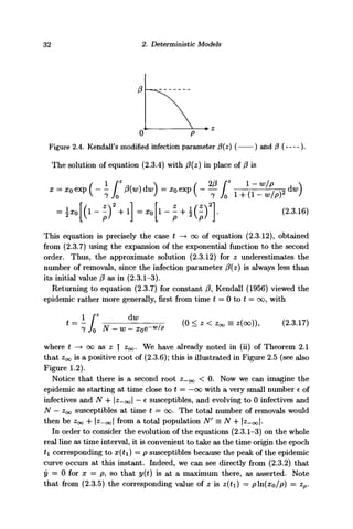
Table 2.2. Characteristics of a general epidemic in terms of the intensity i
Intensity
i
0
0.2
0.4
0.6
0.8
0.9
0.99
Relative size
N'/P
1
1.1157
1.2771
1.5272
2.0118
2.5584
4.6517
Peak incidence
y'(o)/N'
0
0.0056
0.0254
0.0679
0.1556
0.2418
0.4546
Severity before peak
4o/(l*'-<J+4o)
(0.5000)
0.5094
0.5212
0.5379
0.5657
0.5921
0.6662
Notes. For given i, N'/p = | ln(l - i)/i, y'(0)/N' = 1 - (p/N')[l + ln(N'/p)), and
l*'-ool/(*~ + KoJ) = (P/N'i) WN'/P) = [ln(N'/p)]/| In(l - i)|. See text.
region of the critical threshold size p, most of the population is affected (i.e.
a large major outbreak occurs) as soon as N' is 3 or more times p.
Table 2.2 can also be used to relate the measures (#o,2/o) m t n e
original
time scale t to the 'standardized' measures of the table. For, supposing
that (a?o, Vo)i P a n
d N are given, then we can solve equation (2.3.5) to find
the value zp for which xo — p, namely zp = pn(xo/p)y and hence obtain
z' = z — zp. Then z-co and z^ are the two roots of
N - z - xoe~z/p
= 0,
and finally N' = N 4- |^-oo|- All the quantities of Table 2.2 can now be
found.
For example, (a?0, yo) = (800,100), N = 900 and p = 390 gives zp = 280.2,
z-oo = -78.6, z^ = 796.1, so AT' = 978.6 and z = (78.6 4- 796.1)/978.6
= 0.8938, i.e. close to 90% of the population are infected by the epidemic.
Note that the epidemic is skewed about the central value zp in the ex-
ample just given, z^ = z^ - zp = 796.1 - 280.2 = 515.9, while -z^^ =
z-oo ~ zp = 78.6 4- 280.2 = 358.8, which is about two-thirds of 515.9. The
corresponding values of the susceptibles x' are x'^ — 103.9 and x!_oo —
978.6. The value v discussed after (2.3.14) could be estimated as either
800-390 = 410 or 390-103.4 = 286.6, again differing appreciably. In other
words, in terms of Xo = p+v, the rough approximation x^ « p—v — x$ — 2v
holds at best for a small range of intensities i
2.4 The general epidemic in a stratified population
A major aim of this section is to indicate how Kermack and McKendrick's
results as stated in Theorem 2.1 extend to the more general setting of Sec-
tion 2.2 in which an epidemic spreads in a stratified population (hence,

48. 36 2. Deterministic Models
non-homogeneous). We do not need to specify here the basis of the stratifi-
cation: it may be spatial (i.e. geographical), behavioural, cultural or socio-
economic, for example. In this section, in addition to the pairwise infectious
contact rates 0ij for an infective in the ith sub-population or stratum to
infect a susceptible in the jth stratum, for i, j = 1,..., m, we also suppose
that there are per capita removal rates jj for the removal of infectives from
the jth stratum; Zj(t) denotes the cumulative total of such removals by
time t. Then by analogy with the basic equations (2.4.1-3), again by the
Law of Mass Action, we have the differential equations (d.e.s)
Vj = + • • •+
(2.4.1)
(2.4.2)
(2.4.3)
for each j = l,...,ra, with initial conditions (XJ,yj,Zj)(0) = (xjo,yjo,fy-
These equations are expressed more compactly using vector notation similar
to that of Section 2.2, extended to include the vectors
x =
X2
y =
2/1
2/2 Z2
7 =
7i
72
We indulge in the same sort of abuse of notation for lnx as with lnU in
(2.2.6), and extend it to the use of diag7-1
= diag(7f 1
,7^"1
,... ,7^*) for
the diagonal matrix whose elements are the reciprocals of the elements of
a vector like 7. In this vector notation, with B = (A?)? the differential
equations (d.e.s) (2.4.1-3) are expressible as
x = - diag(x)B;
y, y = diag(x)B'y-<iiag(7)y, z = diag(7)y. (2.4.4)
Writing B7 = B'diag(7~1
), the first and third of these give (cf. (2.3.4))
dlnx . , . 1x
—r— = -B /
diag(7"1
)z = -B7 z.
Integration on (0, t) coupled with the initial conditions leads to
j - 1, •..,m), (2.4.5)
i=

49. 2A. The general epidemic in a stratified population 37
provided that this solution curve or trajectory lies in the region X defined
by
Xj, Vjy Zj > 0, Xj + yj + zj = Xjo + yjo (j = 1, • ••, m). (2.4.6)
It is not difficult to check that the trajectory does indeed lie in X: it fol-
lows from (2.4.1) that trajectories in X are monotonic in each Xj, and
yj(t) > 0 for 0 < t < co assuming the matrix B is primitive (i.e. for
sufficiently large n, all components of B n
are strictly positive). Then
using the boundedness as well, it follows that the component vectors of
lini£_>Oo(x,y,z) = ( x 0 0
^ 0 0
^ 0 0
) exist and satisfy
y~=0, x ^ x o - f v o - z ~ ,
x? = xj0 exp ( - [B7zoo
]i) (j = 1,..., m).
Thus, the d.e. system (2.4.1-3) yields a unique limit point ( x 0 0
^ 0 0
^ 0 0
) .
Further analysis completes the proof of part (i) of the following statement,
which is an analogue of the Kermack-McKendrick Theorem 2.1.
Theorem 2.2. A general epidemic evolves in a stratified population ac-
cording to the differential equations (2.4.1-3) in the region X, starting from
initial values (xo,yo,0), where the transmission matrix B is primitive and
the removal rate vector 7 has all components positive.
(i) (Survival and Total Size). When infection ultimately ceases spread-
ing, positive numbers of susceptiblcs Xj° remain in each of the strata j =
1,..., m. The numbers of removals Zj° constitute the unique solution in X
of the equations (2.4.7). If Xo is replaced by any XQ that is componentwise
larger than XQ, i.e. XQ >: xo, then z°° is replaced by z/oc
>z z°°.
(ii) (Threshold Theorem). A major outbreak occurs if and only if the eigen-
value Amax of the non-negative matrix diag(xo)B7 with largest modulus,
lies strictly outside the unit circle, where B 7 = B/
diag(7~1
).
(iii) (Second Threshold Theorem). If x0 = f -h Ax, where the components
of Ax are non-negative and sufficiently small and Amax(diag(£)B7) = 1 <
Amax(diag(xo)B7), then
( 2 A 8
)
2=1
~ 1
)i.e. z°° w 2[l'diag(v~1
)(x0 - £)]v, where v is the right eigenvector of the
eigenvalue 1 of the matrix diag(£)B7.
The detailed proof of this theorem can be found in Daley and Gani (1994);
we confine ourselves here to some indicative comments. Watson (1972)
treats special cases of the model.

50. 38 2. Deterministic Models
Equations (2.4.7) can be solved iteratively via the transformation T :
(n
) *—> z(n+1
) defined componentwise by
- expf-CB^W),]), (2.4.9)
starting from any convenient z^0
) e X such as z^0
^ = yo. Thus, the vector
z°° is a fixed point for T, i.e. Tz°° = z°°, and under the stated conditions
it is the only fixed point in X.
The criticality statement (ii) is motivated in part by recalling that for a
general epidemic in a homogeneous population, the initial point (xo,yo) is
close to the singular point (#o, 0) for the pair of d.e.s (2.3.1-2) describing the
evolution of the process. The linear d.e. system approximating (2.3.1-2) at
that singular point either diverges when XQ > p or converges when x0 < p. A
linear approximation to (2.4.1-3) in the neighbourhood of (xo,yo) ~ (xo, 0)
leads to a similar divergent/convergent dichotomy, determined here by the
dominant eigenvalue of the matrix analogous to the product xo/^T"1
of the
Kermack-McKendrick Threshold Theorem. We shall meet Amax again in
Section 3.5 in the context of the Basic Reproduction Ratio.
The approximation in (2.4.8) is derived by a power series expansion in
the solution equations (2.4.7), much along the lines of the argument below
(2.3.14) based on (2.3.5).
The description we have given for an epidemic in a stratified popula-
tion is not the only possibility. For example, Ball and Clancy (1993) and
Clancy (1994) allow individuals to move between strata, hence offering a
more general cross-infection mechanism than our formulation with the ma-
trix B allows. Exercise 2.4 sketches details of a special case of Theorem 2.2,
and Exercise 3.9 evaluates Amax for a special case of B.
Exercise 2.5 discusses briefly the question of stratified population ana-
logues of the 'other' root Z-OQ (see Figure 2.5) and the standardized in-
tensity measure i at (2.3.18). Certainly, B"1
is well-defined when B7 is
primitive.
2.5 Generation-wise evolution of epidemics
One can envisage an infection in a population as spreading along a sequence
of links from any given individual to a number of others. If for example
the infection is 'psychological' like a rumour or item of important news
(cf. Chapter 5), then there may be a strong interest in knowing how many
individuals are infected direct from the initial infective(s): this is the number

51. 2.5. Generation-wise evolution of epidemics 39
of first-generation infectives. Individuals infected first-hand from one of
these first-generation infectives are then second-generation infectives, and
so on through to the j th generation. The accuracy of the 'infection' may
be affected by the closeness or otherwise of the source of an individual's
infection to the initial infective(s). In the case of the simple and general
epidemic models of Sections 2.1 and 2.3 the proportion of j th-generation
infectives can be derived algebraically. To the extent that this involves
considering sub-divisions of the population, there is some overlap with the
analysis in Sections 2.2 and 2.4.
For clarity below and consistency with all of our later exposition, we set
N = x0 and / = yo in notation used up to this point, and N' = N +1.
Consider first the simple epidemic model of Section 2.1. Use yj(t) to
denote the number of infectives at time t who have acquired their infection
by contact with some (j — l)th infective, i.e. with an infective counted
amongst the yj-i(u) infectives of the (jf — l)th generation at some earlier
time u < t, the instant of contact for the individual concerned. So, in
a simple epidemic in a population of size N', there is a constant number
yo = I of initial infectives, yi (t) who by time t have been infected first-hand
from these y0, and so on up to yj(t) j th-generation infectives who by time
t have been infected from the ?/j_i(£).
We assume homogeneous mixing of the population, with the infection
spread from one individual to another. Then, when the size N of the closed
population is large, the equations describing the spread are
j^t) 0 = 1,2,...), (2.5.1)
with
oo
J2 N + I-x(t) = N'-x(t)- (2.5.2)
note that the number of generations j must in fact be finite. In addition to
the equations at (2.5.1) we also have the relation y = (3xy = /3(N'—y(t))y(t)
as at (2.1.1), from which we know that y(t) = IN'/(I + Ne-W*) (see
(2.1.2)).
To solve the d.e.s (2.5.1), rewrite them as
(2.5.3)
so
/
Jo
/ ^ ^ d u j (j = 0 , 1 , . . . ) ,
o Jo

52. 40 2. Deterministic Models
150
100
1 2 3 4 0 5
(a) (b)
Figure 2.7. Growth of 'generations' 0, 1, 2, 4, 6, 8 of infectives in a
simple epidemic with (AT, /) = (1000,1), 0 = 0.0001, on 0 < 0N't < 10;
part (a) is an enlargement of the start of (b). The number at the right-
hand end of the curve shows the generation number; generation 6 is the
modal generation for large t.
where W(Uj) = yiu^/yiuj) = (d/dt) lny(t)|t = u / Thus,
yo(uo)W(uo)W(u1)...W(uj)duodu1...dur
0<uo<ui<-"<u3<t
Here, yo(u) = / (all u > 0), and the (j + l)-fold integral is symmetric in its
arguments, so with
lnU(t)= /V(«)d«= / '
Jo Jo du
we have
(2.5.4)
Equation (2.5.4) shows that the sequence {y3t)} is proportional to the terms
of a Poisson distribution with increasing mean In U(t) (cf. Daley, 1967a).
For small t (meaning, 0N't = o(l)), lnU(t) « (1 - I/N')0Nr
t. Figure 2.7
illustrates the growth of the 'generation sizes' in the case (JV, /) = (1000,1),
0 = 0.0001 and /?AT't < 10. Part (a) of the figure shows the behaviour for
smaller t.

53. 2.5. Generation-wise evolution of epidemics 41
To study the generation-wise evolution for the general epidemic model of
Section 2.3, we continue to use the functions yj(t) as defined above (2.5.1),
and introduce thf function Zj(t) to denote the number of j th generation
infectives removed by time t. In place of the d.e.s (2.5.1), we define t/_i = 0
and now have for j = 0,1,...,
x = -/3xy,
Vj = fayj-i -IVj, (2.5.5)
where y = YlJLo Vjas
before, and y = (f3x — ^)y. Thus, (3x = 7 -I- y/y, and
the second of the equations at (2.5.5) becomes
or equivalently,
Here we have written Wj(t) = eyt
yj(t) (j = 0,1,...) and it;(t) = e
for which u;0(t) = / (0 < t < 00) and Wj(0) = 0 (j = 1,2,...). Setting
VF(t) = dlnu7(£)/d£, we see that the functional form of these equations is
exactly the same as in (2.5.1), with solution
, j ( t ) _
J '
*similar to (2.5.4). Then, since /0* W{u) du = n[w(t)/w(0)] = jt+ln[y(t)/I],
Thus, as for (2.5.4), the relative frequencies of the generation types among
the infectives at time t are proportional to the terms of a Poisson distribu-
tion. However, since from (2.5.5),
.,(.)-7 / * * ( . ) * . - 7 / / ' . - ' • ' 1 t t l a |
; | l ) /
" ' ' < . , (2.5.7)
^0 Jo J '
we see that for the removals at time t, the numbers in the various generations
are proportional to the terms of a mixed Poisson distribution. The mixing

54. 42 2. Deterministic Models
15 2010
(a) (b)
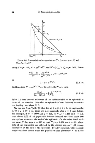
Average generation number among removals in a general
), deaths in a linear birth-and-death process (—•—•—)
Figure 2.8.
epidemic (
and 'aged' infectives in a simple epidemic ( ) with (AT,/) =
(1000,1), (3N't < 20 and (a) 7 = 0.01 (hence, p = 100, Ro = N/p = 10),
and (b) 7 = 0.05 (hence, p = 500, Ro = 2). See Section 3.5 for discussion
concerning the Basic Reproduction Ratio RQ.
factor 7e 1U
du arises from the distribution of the time an individual, once
infected, remains so until it is removed.
As a measure of the average number of generations represented among
the removals we use
Tm(t) = (2.5.8)
The denominator here is z(t) = N +1 - x(t) - y(t) = p]n[N/x(t)], while
the summation in the numerator yields, on simplification,
0
ln[N/x(t)} Jo
*) du. (2.5.9)
This function is conveniently studied numerically by means of the three d.e.s
rh = m (2.5.10)
The function m{t) is plotted in Figure 2.8 together with the corresponding
functions from the simple epidemic and linear birth-and-death processes
(see Exercises 2.6 and 3.5 respectively).
We see that the ultimate 'average' generation number of those infected
in a general epidemic is larger than the corresponding 'average' in a simple
epidemic. This occurs because in the former the number of infectives is
reduced by removal, thereby slowing down the rate of spread of infection

55. 2.5. Generation-wise evolution of epidemics 43
(so, the pool of susceptibles remains larger). Thus the difference in the
ultimate averages reflects the later occurrence of infection in the general
epidemic as against the simple epidemic. These interpretations are further
borne out by the comparison of the two sets of averages for the same initial
conditions and pairwise infection rate, but increased removal rate of (b)
over (a) in Figure 2.8.
It follows from (2.5.7) that Zj° = lim^oo Zj(t) equals the limit as t —•oo
of the given integral. Recall from (2.3.6) that x(t) and y(t) are related by
y(t) = C + plnx(t)-x(t) where C = N + / - pin AT. (2.5.11)
Also, from Kendall's argument referred to following (2.3.17), the monotonic
function x(t) has inverse r(x), given by r(N) = 0 and for N > x > XQQ,
N
dx x_ fN
^__ fN
i~L 0xy"Jx
Writing v{x) = /Q
r
W(u) du, the limit of the integral (2.5.7) after a change
of variable from t to x gives
ao nu-u) ' JXoo 3
(2.5.13)
where
N
Dunstan (1982) used Daley's (1967b) result (2.5.7) to show that for fixed
/ and j and large iV, with N ^$> p,
(2.5.15)
irrespective of the infection and removal rates /3 and 7. This right-hand side
is the same as limt_>oo Vj(t) in the simple epidemic (see (2.5.4)), and hence
is a limit property of {z?°} when p I 0. To explain this coincidence, observe
from the d.e.s at (2.5.1-2) and (2.5.5) that the simple and general epidemic
models with the same initial conditions and pairwise infection rate /?, have

56. 44 2. Deterministic Models
100
30
Figure 2.9. Growth of odd-numbered 'generations' in a general epidemic
on 0N't < 30 with (iV,/) = (1000,/), 0 = 0.0001 and (a) 7 = 0.01
(hence, p = 100, ft, = 10), (b) 7 = 0.05 (hence, p = 500, Ro = 2).
Generation number shown at right.
30
approximately the same behaviour for 0 < t < 0(7 l
/N) =
Then for sufficiently small 7, at the end of this 'initial' phase, the population
in the general epidemic will consist almost entirely of infectives for which
the generation-type will be the same as under the simple epidemic. The
simple epidemic by this time has essentially reached its final state, while
in the general epidemic model each j th-generation infective subsequently
becomes a j th-generation removal.
Let us now review both these results and the properties of birth-and-
death processes (see Exercise 3.5), in conjunction with the fact that for a
discrete time Galton-Watson branching process the mean sizes of successive
generations form a geometric rather than Poisson sequence. We see that
the Poisson nature is attributable to the modelling assumption that any
infective, irrespective of 'age', is as likely as any other to infect a susceptible.
The mixed Poisson characteristic in the proportions of removals, comes from
the delay between an individual's being counted first as an infective and
subsequently as a removal in the general epidemic, or a death in the birth-
and-death process. The fmiteness of the population reduces the average
generation number from a linear function, as in the linear birth-and-death
process, to either In U(t) or /0* W(u) du, both of which have finite limits as
t —• 0 0 .
Figure 2.9 shows how the odd-numbered Zj(t) evolve in general epidemics
for the same models and initial conditions as in Figure 2.8.
Exercise 2.7 sketches another model for the generation-wise evolution of
an epidemic in which successive generations are non-overlapping.

57. 2.6. Carrier models 45
2.6 Carrier models
A major complication with certain diseases such as typhoid, tuberculosis
and poliomyelitis is that the infectives who are the source of infection in the
community, may be individuals who do not display any symptoms and are
apparently healthy. It may take the detection of a geographical pattern of
infection, or a mass screening programme before such infectives are iden-
tified and removed from contact with susceptibles. We call such infectives
carriers to distinguish them from susceptibles who, on being infected, may
be quickly recognized by their symptoms and removed from the population.
This type of situation requires a somewhat different model. The infection
of a susceptible through contact with a carrier, in the simplest model, now
results in the removal of the infected susceptible while the number of carriers
remains unaltered. Carriers are distinct, and their numbers are diminished
by an independent removal process. Applying the Law of Mass Action,
the numbers of carriers w(t) and susceptibles x(t) follow the differential
equations
x = —(3xw and w = —yw. (2.6.1)
These are easily solved, given initial conditions (x(0),u>(0)) = (xo,wo), as
w(t) = woe-^ and x(t) = xoexp ( - (f3wo/j)(l - e~7
*)). (2.6.2)
In practice, when a carrier-borne disease is recognized in a community
where it is normally absent, measures are quickly taken to locate the source
or sources of infection. Suppose then that the introduction into the com-
munity of wo carriers occurs at time t = 0, and that the identification of the
disease through some susceptibles who have developed symptoms occurs at
some time to later, at which point the removal rate 7 increases to 7' say.
The result of such activity is that the d.e. for w is no longer as at (2.6.1)
but
-yw (0<t< to),
(t > to),
while the d.e. for x is unchanged. Then the solution is now that in (2.6.2)
for 0 < t < to, while for t > t0 it is
-={_;,:. :::::'"" (2.6.3)
w(t) = 0
x(t) = x(t0) exp ( - (f3w(to)h')(l - e-^-1 0
))).
Carrier models have a much simpler structure than the general epidemic
model, due to the fact that the process w(t) in the model is independent of
x(t); x(t), however, depends on the evolution of w(t). See also Exercise 2.8.

58. 46 2. Deterministic Models
2.7 Endemicity of a vector-borne disease
The development of epidemic modelling owes much to the work of malariolo-
gists Ronald Ross (1857-1932) and George Macdonald (1903-1967); see e.g.
Macdonald (1973). Malaria, unlike viral diseases such as measles, mumps
and HIV which spread by contact between infectives and susceptibles, is
caused by a parasite whose life-cycle is spent partly in an intermediate
host, the Anopheles mosquito. The mechanism of infection in this case is
different from that which we have so far studied; we must now track the
disease-status of both human and mosquito populations. Our aim is to
model the progress of an outbreak of malaria, and thereby describe condi-
tions for its endemicity. We outline briefly a simple deterministic model,
noting that it is capable of considerable refinement, in both deterministic
and stochastic settings (see e.g. Anderson and May (1991, Chapter 14) and,
particularly, Bailey (1982)).
The life-span of malarial infection is relatively short compared with the
human life-span, and a mosquito population is typically unaffected by the
prevalence or absence of malaria. Thus, it suffices to consider two popu-
lations of constant sizes iVi humans and AT2 mosquitoes, in both of which
individuals are either infected or not, the numbers of susceptibles and in-
fectives being Xk(t) and Yk(t) respectively, Xk{t) + **(*) = Nk (A; = 1,2).
A human infective with malaria loses infectivity (and is again susceptible)
at rate //j; similarly a mosquito infective dies at rate /i2 and is immedi-
ately replaced by a new-born susceptible. A mosquito depends on biting
a human for a blood-meal during which it can ingest infected blood if the
blood-source is malarial; in its turn it will infect a human susceptible when
it is infective (see the cited references for more biological detail). Then the
human malaria-infected population, neglecting any latent period, changes
at rate
and similarly, for the I2W malaria-carrying mosquitoes,
where j3 denotes the feeding rate per mosquito and 7^ the infection trans-
mission rate from an infective of type i to a susceptible of type j (i, j = 1,2).
In terms of proportions xk = Xk/Nk = 1 — yk (k = 1,2),
jV2
V = 0l2ij^V2Xi - /Ziyi = fii(a1y2x1 - 2/1),
2/2 = /? ( )

59. 2.7. Endemicity of a vector-borne disease 47
0.5
(a) threshold just exceeded
0 0.5 1
(b) threshold well exceeded
Figure 2.10. Level curves 2/1 = 0 and 2/2 = 0 in the 2/1-2/2 phase-plane.
where ax = /?72i(N2/Wi)/Mi, a2 = £712/A*2- By inspection, 2/1 = y2 = 0 is
a stationary point, as is any solution of the equations 2/1 = 0 = 2/2 > namely
Thus
2/1 = a i 2 / 2 ( l - 2 / i ) and 2/2 = <*22/i(l - 2/2).
2/2 = (2.7.2)
is a possible equilibrium value; it always lies in (—00,1), and in (0,1) if and
only if aic*2 > 1, i.e.
£-* < ^rN
>- (2
-7
-3)
£>721 V>2
Thus, according to the model, if malaria is to remain endemic a threshold
condition must be satisfied, namely that the relative recovery rate of humans
from malarial infection must be smaller than the relative infection rate of the
new-born mosquito population. Further, as also noted by Ross (1916), to
eradicate malaria, it suffices to reduce the mosquito population sufficiently.
Macdonald (1952) distinguished two types of behaviour of infected popu-
lations where malaria was endemic: in some populations malarial infection
would ebb and flow quite markedly ('unstable' endemic), while in others
it would remain at an approximately constant level. Sketching the curves
T/i = 0 and 7/2 = 0 from (2.7.1) in the 2/1-2/2 plane, and supposing that
the system lies above the threshold as at (2.7.3), these curves cross at the
stationary point at an angle lying between zero and a right angle. The first
extreme, where the curves cross at a small angle, corresponds to a situation
where the infection and transmission levels are only just sufficient to yield
an endemic situation: small changes in the level of one of 2/1 and 2/2 (in Fig-
ure 2.10 it is 2/2, i.e. the fraction of the mosquito population that is infected)

60. 48 2. Deterministic Models
determine large changes in the equilibrium level of the other. Under these
circumstances the disease, while endemic, is still subject to large changes
in infectivity resulting from relatively small changes in the infestation level
of the mosquito population. The second extreme corresponds to the case
where a significant change in the level of either y or 1/2? determines a sig-
nificant change in the other; this corresponds to an endemicity whose level
is sustained quite steadily.
2.8 Discrete time deterministic models
All data available for epidemics are gathered at discrete time intervals, as for
example the numbers of infectives recorded in a population on consecutive
days, or in consecutive serial intervals. It is therefore proper to examine the
principles of deterministic modelling in discrete time, whether as skeletons
of continuous processes or as discrete processes in their own right.
Gani (1978) studied a discrete time equivalent of the simple epidemic,
where observations are made at the times t = 0,1,... . Let a closed popu-
lation of size N consist of xt susceptibles and yt infectives at time t where
%t + Vt = N and yo is given, with 0 < y0 < N. One way of describing the
progress of a simple epidemic, appealing to the Law of Mass Action, is by
the difference equation
yt+i = mm(yt + (3yt{N - yt), N) (t = 0,1,...), (2.8.1)
where /3 represents the pairwise infection rate over the discrete time unit
concerned; this parameter is usually different from that for the analogous
model in continuous time. Omitting the min(-) operator and expressing the
relation in the form yt+ — yt = /3yt(N — yt) stresses the analogy with the
logistic equation (2.1.1) for population growth.
We study the process {yt} through the function
f(y) = /^(/r1
+ N - y) = y + f3y(N - y) (2.8.2)
which is concave, /(/3"1
) = N = f(N), and has 0 and N asfixedpoints. We
use this function because, at least for 0 < yt < min(iV, Z?"1
), yt+i = f(yt)-
Define a sequence {yf} by y% = y0, yt*+1 = f(y$) so that yt = yt provided
the right-hand side lies in the range (0, N). There are two cases to consider,
according as f3N < 1 or (3N > 1. In the former case, this discrete time
epidemic parallels the behaviour of the simple epidemic in continuous time
as presented in Section 2.1 above. To see this, note that f(y) is a parabola
as shown in Figure 2.11 (a), and that for y < N, y < f(y) < N. Thus,
starting from positive y0 < N, y$ < N < 1//3 for alH = 1,2,... so yt = y*,
and yt | N as t —• 00.

61. 2.8. Discrete time deterministic models 49
N
(a) PN < 1 (b) 0N > 1
Figure 2.11. Discrete time logistic epidemic.
When (3N > 1, it follows from (2.8.2) (cf. Figure 2.11(b)) and the con-
cavity of / that if (3~l
< y* < N, then f(y*) > N, while if 0 < y* < /3'1
then (f3N)y* < f(y*). Consequently, for t such that maxo<s<t{y*} < (3~l
,
< 2/t+1, and therefore for some t sufficiently large, t = T say, we
have > (3~l
> ?/f, and thus
Vs =
>
N. This means that for such
(2.8.3)
Thus, for /?iV > 1, the entire population contracts the disease in a finite
time T-hi.
This type of behaviour is expressed formally in the theorem below: there
is no such analogous behaviour of continuous time deterministic simple epi-
demics. The result is a consequence of the discretization of time.
Theorem 2.3 (Threshold Theorem for Discrete Time Logistic Equation).
For an epidemic described by the logistic growth process in discrete time as
in equation (2.8.1) with an initial number of infectives yo in (0, N), either
(a) (3 < N~l
, and at any time t = 0,1,... after the initial infection, a
positive number of susceptibles remains in the population (i.e. yt < N); or
(b) j3 > N~x
and no susceptibles remain after some finite time T -f-1.
Spicer (1979) used a discrete time deterministic model for predicting the
course of influenza epidemics in England and Wales. It is an analogue of the
continuous time general epidemic model of Section 2.3. Let xt, yt denote
the numbers of susceptibles and new infectives on day £, and (3 the pairwise
infection rate as defined at (2.8.1). Removal of infectives occurs daily, with
the proportion ^ of the new infectives on any given day t remaining in the
population j days later. Assume that 0 < ipj < 1 (all j = 0,1,...).

62. 50 2. Deterministic Models
30-
20-
10-
0-
0 8 10 12
Figure 2.12. Weekly deaths from influenza and influenzal pneumo-
nia in Greater London, 1971-72. (Data from Spicer, 1979.)
Suppose the epidemic starts with XQ susceptibles and yo new infectives on
day 0. Then using the same Mass Action principle as before, the sequence
{(xt, yt)} evolves according to the law, for t = 0,1,...,
yt+i = f3xt =xt- yt+, (2.8.4)
while the number zt+i of infectives removed on day t is given by
=Yt- {Yt+l -
i=o
Spicer used the estimated proportions ^o,... ,^5 — 1-0, 0.9, 0.55, 0.3, 0.15
and 0.05, with xjjj = 0 for j = 6,7,..., to predict the progress of influenza
epidemics in Greater London in 1958-73, and hence to estimate the number
of deaths (as a proportion of the number of infectives) from influenza and
influenzal pneumonia in that period. The important factor was to obtain
an estimate of /?#o; this was found to range between 4.5 and 7.7 in the
period 1958-73. Figure 2.12 illustrates the quality of the fit of the model to
the data (see also Section 6.1 and Exercise 6.1 below). If we assume that
deaths are proportional to the number of new infections in any week, then
the plotted points and fitted curve of Figure 2.12 are proportional to the
epidemic curve defined around (2.1.4).
Saunders (1980) used a slightly different approach to study the spread
of myxomatosis among rabbits in Australia. After infection, a rabbit goes
through a latent period of about 7 days, followed by an infectious period of
about 9 days during which symptoms can be observed. Nearly all infectives

63. 2.8. Discrete time deterministic models 51
die, so that removals in this case are due to death. The model postulates
that a rabbit infected on day t enters and remains in the latent period until
day t + t—1 (£ = 7). It then becomes infectious on day t + £ and remains
so until day t+£+k-l (fc = 9), after which it dies.
Let ?/i (t) denote the number of rabbits first observed to be infectious on
day t; these were infected on day t — £, and remain infectious and in the
population until day t + k — 1. Hence on day £, the total number of infectives
is
fc-i
y(t) = Y,yi(t-j), (2.8.5)
i=o
since any rabbits becoming infectious before day t — k -f 1 have died by day
t. Starting with XQ susceptibles at time t = 0, the number of remaining
susceptibles at time t is
t+t
iO'), (2.8.6)
while the number of those in the latent state is
i(t + J). (2-8.7)
The total number of rabbits alive on day t is
Saunders used the homogeneous mixing model
£) = (3y(t)x(t) (2.8.8)
with an estimated f3 = 0.0031, £ = 7, k = 9, but the fit of the model proved
unsatisfactory (see Figure 2.13(a)). An improved fit results from using a
population dependent model in which
i.e. (3 has been replaced by a/p(x(t)), on the assumption that each infected
rabbit makes contact with a constant number a of rabbits each day. An
estimate of a gave a = 0.34, and this change with p(n) = y/n, resulted
in better agreement with data, as can be seen from Figure 2.13(b). Saun-
ders also used a goodness-of-fit criterion to discriminate between possible
density-dependence functions p(n) = c, y/n and n, where c is a constant.

64. 52 2. Deterministic Models
120-
100-
8 0 -
6 0 -
4 0 -
2 0 -
U
1 1 1 1 1
0 10 20 30 40 50 0 10 50
(a) (b)
Figure 2.13. Rabbit population affected by myxomatosis: observed
data ( ) and fitted models ( ): (a) homogeneous mixing, and
(b) population dependent model. (Data from Saunders, 1980.)
It is possible to develop a discrete time model equivalent to the general
epidemic model of Section 2.3 in which for t = 0,1,...,
xt+i -xt= fixtyt, -yt= /3xtyt - - zt = ~iyt, (2.8.10)
with Xt + yt -f- zt — TV, and /?, 7 are the infection and removal parameters
which may differ from those in the continuous time model. More correctly,
to avoid negative values of xu one should rewrite the first two of these
relations as
xt+1 = max(0, xt - (3ytxt), yt+1 = yt - >yyt + mm{xu f3xtyt) (2.8.11)
and restrict the value of 7 to (0,1). This model was studied in detail by
de Hoog, Gani and Gates (1979) who derived an analogue of the classi-
cal Kermack-McKendrick theorem, but it is somewhat more complex than
Theorem 2.3; we refer the reader to the 1979 paper for details.
Enough has been said to indicate that while it is mathematically more
convenient and elegant to deal with deterministic models in continuous time,
their discrete time analogues are used fairly often when it comes to analysing
data collected daily, or at other serial intervals. The examples sketched
above are intended to indicate both the usefulness and the complexity of
discrete time deterministic models.

65. 2.9. Exercises and Complements to Chapter 2 53
2.9 Exercises and Complements to Chapter 2
2.1 Mimic the solution of Section 2.2 in the two special cases:
(a) For the simple epidemic model in a homogeneously mixing population of
Section 2.1, put m = 1 and K, = 0 in Section 2.2, and deduce that F(v) = 1.
(b) Suppose m — 2, fin = #22 > P12 > 0 = #21; investigate the solution.
2.2 Suppose that the classification of a population by its disease state (suscepti-
ble, infective, removal) is extended by interpolating a latency state between
susceptible and infectious, with the numbers w(t) in this class at time t sat-
isfying the differential equations x = —fixy, w = fixy — 6wy y = 8w — 72/, and
z = jy. Show that the final size in such an epidemic model coincides with
the general epidemic model at equation (2.3.6), and is independent of 6.
2.3 Use a latency state as in Exercise 2.2 in a model for a simple epidemic, so that
the equations of the model consist of the first two equations (for x and w)
and y = 6w in place of the other two equations. Investigate whether any
solution, parametric or otherwise, is available to describe the time evolution
of such a model.
2.4 In the general epidemic in a stratified population described by the d.e.s at
(2.4.1)—(2.4.3), suppose that the rates fi tJ — fi3 and 7j = 7 (all j). Show that
the solution curve of the d.e.s satisfies
(0)]1/ft
= Mt)/x,(0)]1 / f t
(all t),
and hence that
where Z = X/"Li Z
T ls
^n e u n
iQu e
positive root of
Prove that the dominant eigenvalue of Theorem 2.2(ii) is given by Amax =
£7=1*,o/V7.
[Ball (1985) calls such a process a Gart epidemic after the work of Gart (1968,
1972).]
2.5 Show that the quantities Zoo and z-00 illustrated in Figure 2.5 can be deter-
mined iteratively as limn_+oo z^ and linin-^oo z^~n
~^ respectively, where
s<"+1
> = y0 + Xo[l - exp(-s(n)
/p)],
and z(0)
= 0 and n = 0,1,... . For a stratified population, the first of these
equations has the analogue (2.4.9). Investigate the relations
*<--*> = - [ B - 1
ln[l + (y0 - B<->)/XO] ]„

66. 54 2. Deterministic Models
where ln[] here denotes a vector with components ln[l + (yj0 - z^ n)
)/xj0],
much as below (2.4.4), as a possible analogue of the equation for ^~'n
-1
When zj~oo)
= limn-oo z{
rn)
exists and differs from ^(oo)
= limw.->oo^n)
,
define analogues of i at (2.5.18) by ij = [^oo)
+ l^'^O/ATj where N'j =
Xjoexp(—[B7z^~oo
^]J). As an analogue of zp consider the vector B"1
ln[p]
where ln[p] is the vector with components n[yj/0jj].
2.6 For a simple epidemic model, the analogues of the j th generation removals
Zj(t) in a general epidemic model (cf. (2.5.7)), are the jth generation in-
fectives zs
3(t) who have been in this state for an exponentially distributed
time with mean I/7, i.e. 'aged infectives'. These zs
3(t) satisfy the d.e. Zj =
7(yj ~ z
j) where quantities with superscript s refer to the simple epidemic.
Show that the analogue ms
of the function m at (2.5.8) equals Ms
/zs
, where
Ms
= ^2 •3z
j> illustrated in Figure 2.8, satisfies the d.e.
lny.= 7 M + l n y
2.7 The following is a prescription for using continuous time methods to track
the generation-wise evolution of an epidemic process when the latency period
is large relative to the infectious period, and successive generations of infec-
tives are non-overlapping. Introduce functions {Xn(), Yn() : n = 0,1,...}
satisfying the d.e.s
Xn(tn) = -0Xn(tn)Yn(tn) and Yn(tn) = -^Yn{tn) (t > 0),
together with boundary conditions Xo(0) = N, Yo(0) = I and, for n =
0,1,...,
Xn+l(0) = Xn(00), IWi(O) = Xn(0) - Xn(00) = Xn(0) - Xn +l(0).
In this formulation, 'time' tn runs from 0 to oo while the number of nth
generation infectives declines from Yn(0) to zero; at the same time, the first
generation latent infectives are increasing, and the number of susceptibles
declines from Xn(0) to Xn(oo) through the growth of such infectives. At
in = ooa new time axis tn+1 starts at 0 and the process iterates. The d.e.
for Yn has solution Yn(tn) = yn(0)e~7
*n
and so
ln[Xn(t«)/Xn(0)] = -[0Kn(O)/7](l - e~7t
") -> -/?Fn(0)/7 (tn - oo).
(a) Show that Xc» = limn_>oo Xn(tn) exists and satisfies equation (2.3.7).
(b) Prove that, if / is allowed to vary, then limjio[Yi(0)/>o(0)] = 0N/-y = RO
as in Figure 2.8 and in Section 3.5.
(c) Compare Fo(0)H -Yn(0) numerically with Z0(oo)H -Zn(oo), using
the solution of the generation-wise evolution results in Section 2.5, for some
suitable 0/*y, N and /.

67. 2.9. Exercises and Complements to Chapter 2 55
(d) Interpret the sequence {Zn(oo)} in the context of a discrete time general
epidemic model (cf. discussion at end of Section 2.8 and Chapter 4).
2.8 In the carrier model described by the d.e.s at (2.6.1), suppose that a (small)
proportion a of the susceptibles infected become carriers, so that the second
of the equations is now
dw „ 7 d In x dx
with x and w related by w = wo -f a(xo — x) — pn(xo/x). Deduce that the
number of susceptibles #oo surviving the epidemic is the unique solution of
the equation
a(x0 - Zoo) + wo = plnOro/xoo), ^o > Xoo > 0.
[Observe that with this modification, the carrier model is similar to the gen-
eral epidemic model.]
2.9 Suppose that outbreaks of an epidemic take place in a given region (or village)
each year. Consider how to combine data from several years so as to display
features of the evolution of the disease; how could these data be used to
estimate parameters of a suitable model? As a possible model, assume the
same population size for different years and the same parameters j3 and 7 in
the case of the general epidemic of Section 2.3 or its discrete analogue (cf.
En'ko's work in Dietz (1988), En'ko (transl. 1989), and Exercise 1.3 above).

68. Stochastic Models in Continuous Time
In this chapter and the next, perhaps the most important of this book,
we describe the evolution of an epidemic as a stochastic process. Such a
stochastic approach is essential when the number of members of the popula-
tion subject to the epidemic is relatively small. While deterministic methods
may be adequate to characterize the spread of an epidemic in a large popu-
lation, they are not satisfactory for smaller populations, in particular those
of family size.
We shall use the tools of non-negative integer-valued Markov processes in
continuous or discrete time, retaining much of the approach of the previous
chapter in the dissection of the population. However, we no longer use
continuous functions to approximate the evolution of the epidemic; rather,
we consider a closed population of individuals, each of whom is classified
as either a susceptible, an infective or (except for the 'simple' epidemic of
Section 3.1) a removal. This S-I-R classification1
is possible because we
regard the epochs where individuals change their classification as randomly
determined points in continuous time, or asfixedpoints in discrete time. For
mathematical convenience but with sufficient simplistic realism, we assume
that the processes involved are Markovian. The reader is presumed to have
some familiarity with the elements of Markov processes on countable state
space, as for example in Bailey (1964), Cox & Miller (1965), Karlin & Taylor
1
Waltman (see Waltman and Hoppensteadt (1970, 1971)) introduced this notation to
designate both the possible disease states of an individual, and the possible progression
of disease in an individual; here, it denotes susceptible —> infected —> removed. A simple
epidemic as in Chapter 2 or the first two sections below is an S-I epidemic. For an S-I-S
disease like malaria, a simple model envisages that an individual is either susceptible,
infectious or (after recovery) susceptible again. Superinfection is not allowed in this
simplest version in which individuals are either infected to the same extent, or susceptible;
a variant of this model would allow superinfection. Hethcote (1994) surveys deterministic
models more extensively.
56

69. 3.1. The simple stochastic epidemic in continuous time 57
Xt
N
0 tx tjv-l t^-2 ts £2 ^1
Figure 3.1. The death process {X(t) : t > 0}.
(1975, 1984), Bartlett (1978) or Ross (1983). In this chapter we concentrate
on Markov models of epidemics in continuous time.
3.1 The simple stochastic epidemic in continuous time
A simple stochastic (Markovian) epidemic model in continuous time is one
in which the population consists only of susceptibles and infectives; once
a susceptible is infected, it becomes an infective and remains in that state
indefinitely. Thus, the main features of the simple deterministic epidemic
in continuous time also hold for the simple stochastic epidemic we now
describe.
We suppose that the total population is closed, so that
X(t) + Y(t) = N (all t > 0) (3.1.1)
where X(t) and Y(t) denote the numbers of susceptibles and infectives at
time t, with initial conditions (X, Y)(0) = (N, I) where / > 1. We assume
that {(X, Y)(t) : t > 0} is a homogeneous Markov chain in continuous
time, with state space the non-negative integers in Z2
satisfying (3.1.1)
and N > X(t) > 0. The only non-zero transition probabilities occur for
0<i < N, j = N + I -i and are
Pr{(X,Y)(t ) = (i- l,j+ 1) I (X,Y)(t) = (ij)} = fiij
) - (i,j) I (X,Y)(t) = (ij)} = l-/3ij6t-o(6t),
(3.1.2)
with (X, Y)(i) = (0, Af + /) being an absorbing state; /3 > 0 is the pairwise
infection parameter.
Because of (3.1.1), such a Markov chain is in fact one-dimensional on that
part of Z satisfying N > X(t) > 0, or equivalently, / < Y(t) < N + /, the

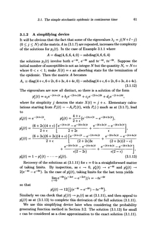
70. 58 3. Stochastic Models in Continuous Time
former being a death process and the latter a birth process on the integers
concerned. This enables us to write down certain properties of the model
fairly easily. For example, concentrating on {X(t) : t > 0} as a pure death
process and referring to Figure 3.1, it is clear that X(-) evolves by unit
decrements at the epochs ts, £/v-i, • • • ,t say, where
N
T
i ( 1 < J < J V ) , (3.1-3)
and the Tj are independent exponentially distributed random variables for
which ETj = l/[/3i(N + I - i)]. Consequently
1 N
1 1 [ N
1 N
~j
1=3 v
/ N(N 4- I -I)
= 1,7=1), (3.1.4)
l n
/ • _ 1 ) / / _ 1 ) + 7/v,/,j otherwise.
x <
Here 7/v,/j = 7iv — 7/-i + 1N+I-J — lj-i with the sequence {77} defined
by
3 1
7o = 0, 7 j = 5 3 T - l n j ( j - 1 , 2 , . . . ) , (3.1.5)
t=i z
and 7j converges as j —> 00 to Euler's constant 7 ^ = 0.577216... Equation
(3.1.4) shows that the mean time Etj until the number of susceptibles is
reduced to j — 1 (j = N,..., 1) can be approximated by the inverse of the
logistic rate (see Exercise 3.1); Williams (1965) and Bartholomew (1973,
Chapter 9) give further comparisons. See Exercise 3.2 for varti when / = 1.
3.1.1 Analysis of the Markov chain
We now analyse the Markov chain {X(t) : t > 0} by the usual methods,
given that the only non-zero transition probabilities, for 1 < i < N, are
Pr{X(t + St) = i - 1 I X(t) = i}= /3i(N 4- / - i)St 4- o(6t),
Pi{X(t + ft) = t I X(t) = i} = 1 - p%(N + / - i)St - o(6t),

71. 3.1. The simple stochastic epidemic in continuous time 59
with X(t) = 0 being the absorbing state. Then the forward Kolmogorov
equations for the state probabilities pi(t) = Pr{X(t) = i X(0) — AT},
(0<i< iV), are
pN = -/3NIpN(t),
Pi = -0i(N + / -
(o.l.o)
where p = —. In matrix terms, for P(t) — (PTV(£), - • •,Po(t))', P = —-Tr-
ot dt
equals
( NI
-NI (N •
-(JV-1)(I + 1) (AT-2)(7
-1) Oj
PN-l(t)
PN-2(t)
Po(t)
so that
P = -0AP(t). (3.1.7)
Here the square matrix A of order N + 1 is the difference of two matrices,
one diagonal and the other subdiagonal:
A = diag(JV7, (N - 1)(7 + 1),..., 1(7 + N - 1), 0)
- subdiag(AT7, (N - 1)(7 4-1),..., 1(7 + N - 1)).
Note that both the diagonal and subdiagonal matrices may have repeated
elements, as in Example 3.1.1 worked out shortly.
The solution of this matrix equation (3.1.7) is known to be
P(t) = e-^P(O), P(0) = (1,0, • ••,0)' = eN+1, (3.1.7')
but explicit results may not be easy to derive by this method. A much
simpler approach is through the Laplace transforms pi(0) = /o°° e~et
pi(t) dt,
Re(0) > 0, 0 < i < N which, applied to equations (3.1.7), yield
fJo
IJo
- p dt = 0pi(O) = -0i(N + 7 - i)pi(0)
4- f3{i + ){N -f 7 - i - l)pi+i(6), (1 < i < N - 1),
f°° _0tdpo
Jo dt °

72. 60 3. Stochastic Models in Continuous Time
We can express equations (3.1.8) in matrix terms as
0A)P = eN+x (3.1.9)
where //v+i is the unit matrix of order N -f 1, ejv+i is the (N + l)-vector
defined at (3.1.7') and P is the vector of Laplace transforms pt(0) of the
elements pi(t) of P. Equivalently,
PN(0) =
0NV
We can solve for Pi{6) recursively, starting with PN(6) to obtain the result
N
where some factors Q--j3j{N+I—j) appear twice for pi(6) with z < ^(
Example 3.1.1. To illustrate the procedure, suppose that (N,I) = (4,1),
13=1. Then
4 ' iy
"v ;
(0 + 4)(0 -f 6) ' Fzy
> ~ (6 + 4)(0 -f 6)2
'
(fl + 4)2
(0 + 6)2
0 '
Note the double factors in pj{6) for j = 0,1,2. Inverting these Laplace
transforms shows that for all 0 < t < oo,
6 ( e e 2 t e ) ,
= 36( - e"4
< + te~4t
+ e"6i
+ te"6
'), ( j
= 1 + 27e~4t
- 36^e~4t
- 28e~6t
-
For details of similar calculations see Bailey (1963; 1975, Chapter 5).

73. 3.1. The simple stochastic epidemic in continuous time 61
3.1.2 A simplifying device
It will be obvious that the fact that some of the eigenvalues A^ = j(N+I—j)
(0 < j < N) of the matrix A in (3.1.7) are repeated, increases the complexity
of the solutions for Pj(t). In the case of Example 3.1.1 where
A = diag(4,6,6,4,0) - subdiag(4,6,6,4)
the solutions Pj(t) involve both e~4t
, e~m
and £e~4t
, te~6t
. Suppose the
initial number of susceptibles is not an integer N but the quantity N€ = N+c
where 0 < e < 1; make X(t) = e an absorbing state for the termination of
the epidemic. Then the matrix A becomes
Ae = diag(4-fe,6 + 2e,6 + 3e,4-h4€,0)-subdiag(4H-e,6-|-26,6+ 36,4-h4€).
(3.1.12)
The eigenvalues are now all distinct, so there is a solution of the form
p)(t) =aje-W + bje-^2t
+Cje-(2+e
^ + d3e~^A
where for simplicity j denotes the state X(t) = j -f- e. Elementary calcu-
lations starting from Pe(t) = —AePe{t), with Pe(-) much as at (3.1.7), lead
to
e -<4
+* p%{t) =
(6 + 2c)(4 + e) ( )
J'
(6 + 3c)(6 4- 2c)(4 + c)
Pi W ^-7-:
(2 + 2e)3e (2-f2c)(2-c)
e-(6+2c)t _ e -
(3.1.13)
Recovery of the solutions at (3.1.11) for e = 0 is a straightforward matter
of taking limits. By inspection, as e —• 0, p(t) —•> e~4
* and p|(£) —>
2(e~4i
— e~6t
). In the case of p|W> taking limits for the last term yields
lim e~6t
(e~3€t
— e~2et
)/e = —te~ 6
*
so that
- e ) - te~6t
).
Similarly we can check that p(t) —> pi(t) as at (3.1.11), and then appeal to
pe
0(t) as at (3.1.13) to complete this derivation of the full solution (3.1.11).
We use this simplifying device later when considering the probability
generating function method in Section 3.2. The solution (3.1.13) for small
6 can be considered as a close approximation to the exact solution (3.1.11).

74. 62 3. Stochastic Models in Continuous Time
3.1.3 Distribution of the duration time
A quantity of some importance mentioned earlier is the duration time t of
the epidemic (see Figure 3.1); it equals the sum
N
Tj (3.1.14)
of N independent exponential variables, each with its own parameter
The Laplace-Stieltjes transform2
of Tj equals
so that if t has the p.d.f. /i(£), then
jff .-AM* =
This p.d.f. is related to the state probabilities pj(-) at (3.1.7) by
fx(t) dt = px(t) /3(N + / - 1) d«, (3.1.16)
so for example when AT = 4, I = 1 and ^ = 1 as in Example 3.1.1,
/i(t) = 4 x 36[-e~4t
+ te"4t
+ (1 + *)e~6
'],
and thus t has the distribution function
Fx{t) = 1 + e~4
*(27 - 36t) - e"6t
(28 + 24t). (3.1.17)
Kendall (1957) used the transform at (3.1.15) to obtain the limit distri-
bution of ^i in the case /?= 1, / = 1, N —> oo. Using the transformation
W = (AT + 1)*! - 2 In N, (3.1.18)
2
We distinguish between the Laplace-Stieltjes transform E(e~0X
) — J°° e~0x
dF(x)
of a random variable X with distribution function F(-), and the Laplace transform
Jo e~^t
p(t)di of an integrable function p(-). They coincide when F has a p.d.f. /(•).

75. 3.2. Probability generating function methods for Markov chains 63
it follows from (3.1.15) that, with /(•) denoting thep.d.f. for W,
•-«-)*-"""II ( > ^ "- jf
}2
ft (l + ")"1 [T(l + 0)}2
(N - oo); (3.1.20)
here Euler's formula r(H-z) = zT{z) = Iim7v—oo N z
f l ^ i W + {z
lJ)] l
(e
&-
Whittaker and Watson, 1927, p. 237) justifies taking the limit. Inversion of
the Laplace transform [F(l 4- 6))2
leads to
f(w) = 2e~w
K0{2e-w/2
), (3.1.21)
where Ko(-) is the modified Bessel function of the second kind of order zero
(see Exercise 3.3).
This limit distribution for t is interesting as an example of a sum of in-
dependent non-identically distributed r.v.s having a non-Gaussian limit dis-
tribution. This is not surprising, for the components in the sum at (3.1.14)
are certainly not uniformly asymptotically negligible. These components
can be grouped into three phases, so that the sum t consists of a starting
phase of the epidemic where the first few Ti,T2,... have means that are
O(l/iV), then a middle phase consisting of most of the N r.v.s Tt, when i
is not close to either 1 or AT, with means that are O(l/iV2
), and an ending
phase with the last few T/v,T/v_i,... when the means are again O(l/N).
Daley, Gani and Yakowitz (2000) use this three-phase decomposition of t.
An analogue for the general epidemic is indicated in Exercise 3.13.
3.2 Probability generating function methods for Markov chains
An alternative way of studying a Markov chain {X(t) : t > 0} on the non-
negative integers as state space, is through the analysis of the probability
generating function (p.g.f.)
N
<p(z,t) = E(zx
M) = Y^ P f
{*(0 = 3 I X{fy}zj
(M < 1), (3.2.1)

76. 64 3. Stochastic Models in Continuous Time
where 0 < X(t) < N. It is usually possible to obtain a partial differential
equation (p.d.e.) for (p(z,t) from the Kolmogorov equations for the prob-
abilities for X(t), at least when the transition rates are simple polynomial
functions of the non-negative integers as is often the case in models of pop-
ulation processes. In some cases the p.d.e. admits an explicit solution. We
consider the Markov chain for the simple epidemic of Section 3.1 to illustrate
the method; we shall use the technique again in Sections 3.3 and 3.6.
We use the forward Kolmogorov equations (3.1.6) for the probabilities of
X(t) taking values in 0,..., AT, but first simplify them by changing the time
scale so that the new time t' = (3t. Then since
equations (3.1.6) are replaced by the same relations with (3 = 1 and t'
in place of t. For convenience below, we write t = tf
. Now multiply the
equation for dpj/dt by zj
and sum over j . Writing
£(«)*', with v>(z,0) = ^ and ^ M = £ &&
j=0
this gives
j=o
where PJV+I = 0. Simplifying the sums yields
(3.2.3)
If we differentiate (3.2.3) with respect to z and let z | 1, we deduce that
^ ^ = E(X(t)[(X(t) - 1]) - (N + 1 - l)EX(t), (3.2.4)
so with & = EX(t),
Recall from (2.1.1) that for the deterministic model of a simple epidemic,
with the change of time scale used here, the function x(t) denoting the
number of susceptibles at time t satisfies
x = —x{N + I — x).

77. 3.2. Probability generating function methods for Markov chains 65
Consequently, since x(0) = £o = ^(0)> EX(t) « #(£) so long as vanX(t) is
small relative tox(N+I — x). But, it should be noted that the deterministic
results do not necessarily approximate the mean of the stochastic model well
for all t.
We can solve the second-order p.d.e. at (3.2.3) by the standard method
of separation of variables. This means writing <p(z, t) = Z(z)T(t) for some
functions Z and T, in which case (3.2.3) becomes
-I-l)— = -X say, (3.2.5)
where
= dZ(£) „= d2
Z(z) . = dT(t)
dz ' dz2
' dt
and A is a constant. The simpler relation at (3.2.5) gives T = —AT, so
that T = e~At
. However we know from Section 3.1.2 that this result will be
correct only if the initial number of susceptibles N is replaced by Ne = N+e
(0 < e < 1) in the eigenvalues of the matrix A of (3.1.7). Assume this is
done: then from the rest of (3.2.5),
z{ - z)Z" - (1 - z)(Ne + / - )Z' -Z = 0. (3.2.6)
This is a hypergeometric differential equation of the general form
z( - z)Z" + [c - (a + 6 + l)z]Z' - a&Z = 0,
where c = 1 — (ATe + /), a + 6 = — (iVe -f /), a& = A. A suitable solution of
(3.2.6) is known to be the hypergeometric function
Ziz) -[Z)
^ r(a)r(b)T(c+k)k
The eigenvalues Xj must be such that F(a, 6; c; 2) is a polynomial in z of
degree not greater than iV, which means that a or 6 must be a negative
integer such that a + b = —(Nf + /) is satisfied. Thus the Aj must be of the
form
A, = j(Ne + / - j) (0 < i < TV), (3.2.7)
with a = —j say and b = — (iVf + J — j). It follows that
TV
y>0M) = ^ a
i e
~ J
' ( N e + 7
" J )
^ ( - ^ i - AT, - /; 1 - iVe - /; z), (3.2.8)

78. 66 3. Stochastic Models in Continuous Time
where the coefficients a7 can be obtained from the initial condition
N
(p(z,0) = zN
= J2a
JF
(~JJ - Ne - 7; 1 - N€- 7; z)
3=0
and certain orthogonality conditions satisfied by the functions i?
(-,-; *; z).
If we now let e —» 0, so Ne —> iV, we recover the exact solution to (3.2.4).
Bailey (1963) gives full details of this solution in the case 7 = 1.
Clearly, while this result may be satisfying analytically, it is not easy
to use in practice. Nevertheless p.g.f. methods can be useful, especially in
condensing equations from which summary information like moments can
be deduced.
3.3 The general stochastic epidemic
We consider next an S-I-R model in which the total population N + I
is subdivided into X(t) susceptibles, Y(t) infectives and Z(t) immunes or
removals, with (X,F,Z)(0) = (AT, 7,0) and
X(t) + Y(t) + Z(t) = N + I (all t > 0). (3.3.1)
We assume that {(X, Y)(t) : t > 0} is a bivariate Markov process; (3.3.1)
ensures that Z(t) = N + I — X(t) — Y(t) is known when (X, Y){i) is known.
We again assume that there is homogeneous mixing so that in the time
interval (£, t + 6t) infections occur at rate /3ij6t and removals at rate
yielding for the infinitesimal transition probabilities
Pr{(X, Y)(t + 6t) = (i - 1, j + 1) | (X, Y)(t) = (ij)} = pijSt + o(6t),
)(t + St) = (ij - 1) | (X,Y)(t) =
, y)(t + «) = (i, j) | (
where /? is the (pairwise) infection parameter and 7 the removal parameter.
Then if we write the state probabilities as
Pij(t) = Pr{{X,Y)(t) = (i,j) I (X,Y)(0) = (AT,/)}, (3.3.2)
we can readily derive the Kolmogorov forward equations in the form
(0 < i + j < N + 7,0 < i < N,0 < j < N +1),

79. 3.3. The general stochastic epidemic 67
subject to the initial conditions PNI(0) = 1, Pij(O) = 0 otherwise. Note for
later use that the distribution {Pn} of the ultimate size of the epidemic,
meaning, the distribution of the number of initial susceptibles ultimately
infected, is given by
Pn = Pr{ lim (X, Y)(t) = (JV - n, 0) | (X, Y)(0) = (N,I)} = P7v-n,o(oo).
t—+00
This distribution is computed most efficiently, in terms of time, numerical
precision and range of values of N + /, via an embedded jump process: see
Section 3.4.2 and Figure 3.2.
Some slight simplification is achieved if we define tf
— /3t so that d/dt =
/3d/dt' much as before at (3.2.2). With p = 7//? as the relative removal
rate, the equations (3.3.3) become (again writing t = t1
for convenience)
^ | W = {i + 1){j _ i)ps+1J .1 _j{i + p)pij
(0 < i + j < N + /, 0 < i < N, 0 < j < N + /),
subject to the same initial condition PNI{Q) = 1- We could now attempt to
solve these equations recursively, starting with PNi{t) = e~(N+p>)It
. Such
a procedure is tedious (see Exercise 3.4), and it is preferable to use a sys-
tematic approach such as one based on a mixture of Laplace transform and
p.g.f. methods. Such solutions were offered around the same time by Gani
(1965, 1967), Siskind (1965) and Sakino (1968): we outline Gani's solution
of 1967.
It is worth remarking that these solutions are possible here, essentially
because the processes concerned are Markov chains with well-ordered sample
paths. The states (i,j) for {(X, Y)(t) : t > 0} have an hierarchical structure,
with the value of X declining by single units, and the value of Y increasing
or decreasing by single units also. The process is 'strictly evolutionary':
once a state is visited and left, it cannot be revisited, so, each state (i,j) is
entered either once or not at all. The forward Kolmogorov equations (3.3.3)
relate the derivative of any given state probability, to state probabilities for
that state and the states immediately preceding it along any well-ordered
sample path. See also Section 3.4.2 and Exercises 3.6 and 3.7.

80. 68 3. Stochastic Models in Continuous Time
3.3.1 Solution by the p.g.f. method
Multiply the respective equations in (3.3.4) by zl
w^ and sum them over i and
j . Then for the p.g.f. (p(z, w; t) of the bivariate Markov process {(X, Y)(t) :
t > 0} denned by the sum
£ (x, r)(o) =
0<i<N
we obtain the p.d.e.
with <p(z,w;0) = zN
w1
. Differentiation of (3.3.5) with respect to z or w
followed by putting z = w = 1 yields (in the original time scale)
-0cov(X(t),Y(t)),
Pcov(X(t),Y(t)),
respectively. Neglecting the covariance terms and putting (x(t),y(t)) =
(EX(t), EY(t)) yields the d.e.s. of the deterministic model of Section 2.3.
Equation (3.3.5) is more simply studied in terms of its Laplace transform
/•OO
(p(z, w;0)= / e~et
ip{z, w; t) dt (Re(8) > 0)
(3 3 7)
7(M)
=
E E0<i<N 0<j<N+I-i 0<i<N
where
Taking Laplace transforms of (3.3.5) yields
0<p(z,w;O) - 2 W =
, Pn(0)= e-et
Pij(t)dt.
Substituting for <p(z,w;9) from (3.3.7), we deduce the set of equations
p)w~p}^,
dw
, (3.3.8)

81. 3.3. The general stochastic epidemic 69
These equations can expressed succinctly in matrix form as
A — + 0F = u/e7v+i, (3.3.9)
where F = (f^ //v-i • • •/o)' and e^+i is the (AT -f l)-row vector with 1 in
its first row and zeros elsewhere, as at (3.1.9). With IJV+I denoting the unit
matrix of order N + 1, the square matrix A = A(w) of order N -f 1 equals
—p(l — W)IN+I +wdia.g(N,N — 1,..., 1,0) — u>2
subdiag(AT, N — 1,..., 1)
= -pljv+i 4- wA'(O) + w2
A"(ti). (3.3.10)
Since each component of the vector F is a finite series in w, F has a finite
Taylor series expansion
N+I j
F(w;0) = Y^ — FiJ
O;0), (3.3.11)
where F^^(0; 0) is the jth partial derivative of F{w; 0) with respect to w at
w = 0. Then setting w = 0 in (3.3.9) we have for / > 1
or
F'(O;0) = (0/P)F(O;0). (3.3.12)
Differentiating (3.3.9) with respect to w yields
[A'(w) + dlAr+^F'^jfl) 4- AHP"(ti;;fl) - Iti/^eAr+r, (3.3.13)
setting t/; = 0 and rearranging gives
F"(0; 9) = - ([A'(0) + 91N+1}F'(0; 6) - I6ueN+1), (3.3.14)
where ^1/ is the Kronecker delta and A'(0) = diag(A^, TV - 1 , . . . , 0)+pIN+1.
Differentiating (3.3.13) leads to
A"(w)F'(ti;; 9) + [2A'(w) + 9IN+1]F"(w; 9) + A(w)F'"(w; 9)
' 2
(3.3.15)

82. 70 3. Stochastic Models in Continuous Time
so setting w = 0 and rearranging as before, we have
F'"(0; 0) = - [[2A'(0) + 0I,v+i]F"(O;0) + A"(0)F'(0;0) - .I1
*2
'
pi (1 — 2)1P1
(3.3.16)
In general, further differentiation of (3.3.15) with respect to w followed
by setting w = 0 and rearranging, shows that F(J
'+1
)(0; 0) equals
P
(3.3.17)
These equations yield a first-order recurrence relation when expressed in
the matrix form
f Fk+1
)(0;6>n9
{ F<»>(O;0) J
A'(O) + «Af+i (J
2)A"(0)^j f FO)(0;e) ^j I6jt (eN+1)
plN+i 0 J lpW-D(0;^)J (/-j)! I 0 J'
(3.3.18)
this relation is valid for j = 0,1,..., N + I when we define F<0)
(0; 9) =
F(O;0), F<-1
)(0;«)=0.
We see that for j = 0 , . . . , / - 1,
where for k < j we define the product Jl^fc ^* =
EjEj-i • ••Bfe+iBfc. For
j = /, however, we have
and for j = 1 + 1 , . . . , / + AT,
r FC+^O^) 1 _ rrB . f F(o;*) ^| /! r ew+1)
I F(')(0;») J ~l= lB l
I 0 J 7 1 0 J' (3
-3
-19
)
i—0
F(O;0)^| /! A few + 1 )
0 J ~ 7 11Bi
[ 0 J (3
-320)

83. 3.3. The general stochastic epidemic 71
Since
(F
F
Hence,
p(JV+7+l)(()
AT+7+l)(0;e)
^N+/
)(0;6>)
i=0
)
0
= 0, it follows that
)) /' N+I
(
[
iV+7 -i y, r iV+7 -I
nBi
j 1
F ( O ; 0 ) =
7[ nBi
jwhere [*]JV+I denotes the truncated (N + l)-square matrix consisting of the
first TV + 1 rows and columns of its argument. Now from (3.3.18), because
jA'(Q) -f 0IJV+I is a diagonal matrix and A"(0) is a subdiagonal matrix,
both with non-zero elements, any product n i = o ^ ls a
l°wer
triangular
matrix with non-zero eigenvalues for Re(0) > 0. Hence its inverse exists,
and thus
(3-3-21)
Thus, a complete solution of the general stochastic epidemic, in the sense of
describing the Laplace transforms of the state probabilities of (X(t),Y(t))
for finite t > 0, is given by
w,9) ) _N
¥f1
w* ( FW(O;0)
«; 9)dvj- j ^ J ( PW-D(O; 9) J
F(w,9) (3
-3
"22)
WJ
In*-1
* 1 fF(0; e)
) T ' W J n
[n^1
B 1 fejv
+!Z. f P J [ o J .
with Bi as defined at (3.3.18) and F(O;0) given by (3.3.21).
Example 3.3.1. Gani (1967) illustrates this solution for the simplest case
(iV, /) = (1,1), from which it is clear that the solution is not easily calculated
in practice for larger N or /. First we have
J),

84. 72 3. Stochastic Models in Continuous Time
The matrices B; are given by
( 9 0 0 0
0 0 0 0
p 0 0 0
0 p 0 OJ
so the required products are
(6(1
P
0
0
p6
0
f l + p + 0
0
9
0
0
0
P
-2p0
p2
BiB0 =
p0(l
0
According to (3.3.21) this yields
P(O;0) = [B2B1B0]^1
[p-1
B2]2eiV+i
0
p0
0 0 0
p + 0 0 0
0 0 0
p 0 0J
0 0
-2 0
0 0
0 0
0 0
0 0
0 0
0 0
) 0 0
0 0
0 0
0 0J
p + 6){2 + 2p + 6){p + 0){2p + 6)
6{p + 0){2P + 6) 0
2p6 0(l + p
P
) (2 + 2p + 0^
0)) { 0 J
1 . (3.3.23)
The full solution to the 2-person epidemic may now be obtained from
(3.3.22) as the upper left 2 x 2 matrix in
so F(w; 9) equals
0
8(1 +p + 6)
2
)
(3.3.24)

85. 3.3. The general stochastic epidemic 73
This Laplace transform solution is more than enough to indicate that
the form of the time-dependent solution to the problem of describing the
evolution of a general stochastic epidemic is algebraically formidable, at
least with pen and paper (see also Exercise 3.4). Fortunately a composite
picture of such stochastic development is possible; we concentrate on the
ultimate behaviour of the epidemic process, first with the analogue of the
Kermack-McKendrick threshold theorem, and then with a description of
the ultimate size of the epidemic.
3.3.2 Whittle's threshold theorem for the general stochastic
epidemic
One may well ask whether there is a stochastic threshold theorem similar in
nature to the Kermack-McKendrick theorem for the deterministic general
epidemic (part (ii) of Theorem 2.1). We start by considering the case, first
published by Bartlett in 1955 (around equations (19) and (20) of §4.4 of
the first edition of Bartlett, 1978), in which the susceptible population N is
very large, so that
Pr{(X, Y)(t + St) = (i - 1, j + 1) | (X, Y)(t) = (i, j)} « NjSt + o(St)
instead of the exact ijSt -f o(6t), and
Pr{(X, Y)(t + St) = (ij - 1) | (X, Y)(t) = (ij)} = pjSt + o(St).
We write Y(t) for the marginal process of the number of infectives that
satisfies these approximate relations exactly, observing that such a {Y(t) :
t > 0}, with Y(0) — /, is a birth-and-death process with rate parameters
N for births and p for deaths. The p.g.f. of Y is given by
^ pe^-P^jz - 1) - (Nz - p) V
-l)-(NZ-P) 1
*» (3_3_25)
1 - pt(z - 1)
Note that the result for N = p can be readily derived from that forN^p
by setting N = p + e in this case and letting e —> 0. We are interested
in the probability of extinction of Y(i), i.e. in lim^oo Pr{Y(t) = 0} =
lim^oo </?(0, t). Prom the first of equations (3.3.25) we see that the be-
haviour differs between N > p and N < p, namely
< * <" > ")>r=f-i
]imip(0,t)= ' " *~ ~ ' N

86. 74 3. Stochastic Models in Continuous Time
When N = p the second equation in (3.3.25) yields the limit 1, which is
equal to the limit of either of the expressions in (3.3.26). Thus, for N < p,
imt^oo "Pr{Y(t) = 0} = 1 so that the epidemic outbreak is likely to be
small. On the other hand, for N > p, the limit is positive but < 1, so
that the outbreak may be either small or large. Whittle (1955) gave a more
precise analysis of Bartlett's approximation; the essential step is to bound
the number of infectives Y(t) in the actual epidemic process between two
birth-and-death processes like Y(t).
For any £ in (0,1) we can ask whether the intensity of the epidemic,
meaning the proportion of susceptibles who are ever infected, exceeds £. To
this end define
TT(C) = Hm Pr{X(O) - X(t) < NQ = 2 ^ Pn (3.3.27)
with Pn the probability that the final size of the epidemic is n, as given
below (3.3.3). We can bound the component Y{t) in the epidemic process
{(X, Y){t) : t > 0} by F(f) in two bivariate processes
{Y(t), U(t) = I -f X(0) - X(t) : * > 0},
where Y(-) is a birth-and-death process with birth parameter either Ai = N,
as in (3.3.25), or A2 = N(l — C), and with death parameter x — /i2 = p.
Note that £/(£) counts all the individuals who have ever been infected up to
time t, including the initial / infectives. Write
Pjk(t) = Pr{(Y,U)(t) = (j,k) I (Y,U)(Q) = (1,1)},
and
Now the forward Kolmogorov equations for the birth-and-death process with
general birth parameter A are
-£jT = X
U ~ l)Pj-i,*-i -(A + p)jPjk H- p(j 4- l)Pj+i,fc,
(0 < 3 < N + /, / < k < N + /),
defining pjk = 0 when (j, k) lies outside the permissible range. This leads
to the p.d.e.
^ = [Xz2
w -f (A H- p)z + p] ^ , (3.3.28)

87. 3.3. The general stochastic epidemic 75
with the initial condition (f(z,w]0) = zN
w1
. Equation (3.3.28) can be
solved by classical methods. The characteristic equations for Lagrange's
method yield
d(f _ dt __ dz _ dw
~0~ ~ T ~ Xz2
w + ( + p)z + p ~ ~0~'
Denote the two roots of the quadratic equation Xz2
w + (A + p)z + p = 0 in
z by 771 (w), f/2(w)> then
where for 0 < w < 1, rji > 772 > 0. The general solution is thus of the form
<p(z,w;t) =
where g is a function which can be found from the initial condition
Write ^ = 2
—^-, so that z = ^f^ 2
, implying that
T) — Z £ 4" 1
It then follows that
^,»; *) = -7
[^j-^tr1
""2
u4
"^'^ '• (3-3-30)
V y
L {z - r)2)e-Xz{m
-m)t
+ (m -z) J v ;
As t —> 00, the asymptotic distribution of the total number of individuals
ultimately infected is given by
lim <p(l,w;t) = w*4(w) = [ ^ ^ ] ( 1 - /T=~^)/
, (3.3.31)t->oo
where K = 4Xp/(X -f p)2
. We now expand this relation, using Lagrange's
expansion for the function tp(s) = s7
, where s(w) = 1 — y/1 — KW can
conveniently be given as the root S(K) of s2
— 2s + KW = 0 that satisfies
lim^^o s(w) = 0. Note that
s(2 -s) s
w = L — — .

88. 76 3. Stochastic Models in Continuous Time
thus using the formula
for Lagrange's expansion, we see that this leads to
PJX) = lim Pr{U(t) = I + n}= lim Pr{X(0) - X(t) = n}
t—*oo t—*oo
r(2n + J - l ) ! Xn
pn+I
<M-1
n(n + I) (A + p)2«+/ ^ n
^ v
V> ( 3 3 3 2 )
where {Pn(X)} is the probability distribution for the total number of initial
susceptibles ultimately infected, for a specific birth parameter A.
Now we know from (3.3.31) that for N —> oo,
lim < ,1; t) = V Pn(A) = i (A) (P < A)
' (3.3.33)
U (p>A),
so that
f ; [ ( ^ ) ] /
(3.3.34)
n=0
Thus for TV large enough, in the case of an epidemic of intensity £, with
bounding values X = N > X(t) > A2 = N(l — C) for the birth parameters
of the birth-and-death processes involved, we have approximately
n=0 n=0 n=0
or equivalently
(3.3.35)
We can draw the following conclusions from this result.
Theorem 3.1 (Whittle's Threshold Theorem). Consider a general epi-
demic process with initial numbers of susceptibles N and infectives I, and
relative removal rate p. For any C in (0,1), let TT(C) denote the probability
that at most [NQ of the susceptibles are ultimately infected i.e. that the
intensity of the epidemic does not exceed £.

89. 3.4. The ultimate size of the general stochastic epidemic 77
(i) Ifp < N(l - <), then
(ii) IfiV(l-C) <P<N, then
In both these cases there is a probability approximately equal to 1 — (p/N)1
that the epidemic achieves an intensity > C for small (.
(iii) If p > N, then TT(Q = 1, and the probability that the epidemic achieves
an intensity greater than any predetermined £ in (0,1), is zero.
3.4 The ultimate size of the general stochastic epidemic
Various approaches have been used to find the distribution {Pn} of the ulti-
mate size of an epidemic, where in the notation used in and below (3.3.2-3),
Pn=limGPN_nj0(t) (3.4.1)
is the probability that n of the initial susceptibles become infected at some
stage during the epidemic. When there are no more infectives, there are
therefore n + / removals including the / initial infectives. In this section
we indicate two methods of finding this distribution, one as an illustration
of the p.g.f. technique of Section 3.3, the other using an embedded random
walk technique that is much superior numerically, in terms of speed, numer-
ical accuracy and population size that can be conveniently handled. This
method is essentially due to Foster (1955). We give a third method, based
on another embedded Markov chain, in Section 4.5, while other methods
have been used by Bailey (1953) and Williams (1971), as outlined in Bailey
(1975).
3.4.1 The total size distribution using the p.g.f. method
For a Markov process on countable state space in continuous time, the
limiting probability TT^ that the process is in state i can be computed from
the Laplace transform Pi{9) of the probability pi(i) that the process is in i
at time t. The Abelian property
ni = lim pi(t) = lim 0pi(6),
t—•oo 0—»0

90. 78 3. Stochastic Models in Continuous Time
where pi(6) = /0°° e~et
pi(t)dt, yields this probability TT,. In terms of the
generating function fi(w,8) of transforms defined at (3.3.7), this means
that, since for all i, imt-+ooPij(t) = 0 for j =£ 0. then
Pn = lim 0pN-n,o(0) = lim 6fN-n(0,0).
B—*0 0—>0
Thus
Pi
{PN)
= lim 6
f IN (0,9)
I fo(O,0) )
= lim0F(O,6>), (3.4.2)
where F(0,0) is given by (3.3.21). From that equation, recalling that
Bo=
we see that
iV+I / + N
nBA 6F(0,0) =I T Bi
whence, taking the limit as 0 —> 0, we find
AT+I
1 / lim 0F(0,0)
n
N+l
0
(3.4.3)
liV+l
Thus, P = lim^_,o ^^"(0^ 0) equals the right-hand side here pre-multiplied
by the inverse of the matrix product on the left-hand side, where as noted
above (3.3.21), this matrix product is non-singular, with a unique inverse.
The following example indicates what is involved in using this matrix result
in practice.
Example 3.4.1. We compute the distribution of the ultimate size of the
epidemic in the case (AT, /) = (3,1) with p = 1. Setting
= i4 =
1 J
A"(Q)
-2A = -2
(0
3 0
2 0
1 0)

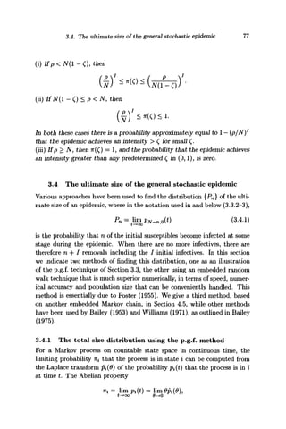
91. 3.4. The ultimate size of the general stochastic epidemic 79
the products appearing in (3.4.3) on the right- and left-hand sides are,
respectively,
(AA -12A) (3A -6A] (2
I / 0 J I / 0 J { I
2A -2A
0
= 24(A3
-AA- AA),
3A -6A
0
( 4A -12A ) f 3
[I / 0 J { I
= 24(,44
-
Hence, after some calculation,
W 2A -2A ( A 0 ^
J ( I 0 J [I Oj
- AA2
- A2
A + A2
).
256
-111
6
0
81
-38
2
• >
16
-7 1,
— x
f64
1-21
0
> 0 >
( 0.2500 >
0.0833
0.1042
w 0.5625 >
p =
Observe the presence here of both positive and negative terms. In larger
matrices this is a source of numerical instability, assuming that there is the
capacity to handle the larger size (e.g. square matrices that are O(100)).
3.4.2 Embedded jump processes
We commented below (3.4.3) that properties like the size3
of the general
stochastic epidemic are most readily studied from a practical point of view
by using an embedded jump chain technique. Aspects of this technique can
be found for example in Todorovic (1992, §8.7); we rehearse here, for the
sake of notation and general convenience, some properties of these processes.
Processes are often modelled as Markov chains because these incorporate
in a simple manner dependence from one time point to another. This is true
for phenomena in both continuous time (as in the earlier part of this chap-
ter) and discrete time (as in the next chapter). In the case of continuous
time, a further class of Markov chains can arise as embedded processes. By
concentrating on the jump points or other epochs of a continuous time pro-
cess which does not necessarily have a Markovian structure, we may derive
a discrete time process which is Markovian (see Section 4.5 for an exam-
ple). For a Markov process in continuous time on a countable state space,
3
The 'total size' of an epidemic usually includes the initial / infectives, whereas
the 'size' (or, 'ultimate size') of an epidemic usually designates the number of initial
susceptibles that are (ultimately) infected.

92. 80 3. Stochastic Models in Continuous Time
the natural process to consider is the one embedded at the jump epochs
of the process. Except for certain pathological cases which do not arise in
the models we have considered, the continuous time and embedded jump
processes both have the same long-term behaviour, such as the development
of major and minor epidemics, and the ultimate size of the epidemic. This
section reviews briefly some results of this kind. The particular usefulness
of embedded jump processes is that they are well-suited to numerical work.
To make these ideas explicit, we use {X(t) : t > 0} in this subsection to
denote a Markov process in continuous time on the countable state space
X = {i,j,...} having time-homogeneous transition probabilities with rates
(Qij)- We assume that X is determined by its initial state and the rates q^
(jf ^ i) and qi = Yli^j Qij ~ ~Q™ (^J ^ ^0- One dichotomous classification
of states is that any state i is either absorbing or non-absorbing, depending
on whether qi — 0 or qi > 0.
Given a sample path for X for which X(0) = i, the time 7$ = inf{£ > 0 :
X(t) ^ i} is well-defined, finite or infinite, with T* < oo a.s. if and only if
qi > 0, i.e. i is non-absorbing. Then Ti is an exponentially distributed r.v.
with mean l/q{. Indeed, supposing without loss of generality4
that the sam-
ple paths are right-continuous with left-limits, these paths can be described
by a sequence of intervals of lengths T^n
with epochs tn determined by the
partial sums
(n = 0,l,...). (3.4.4)
For these,
X(t) = in (tn<t< tn+1, n = 0,1,...), (3.4.5)
for some sequence of states i0, t'i,..., it being understood that if any such
in is an absorbing state the associated interval length T^ is infinite and
tr = oo for all r > n + 1. We can now define the embedded jump chain by
{Xn} = {X(tn + 0):tn< oo}, (3.4.6)
with one-step transition probabilities for non-absorbing states i
Pij = Pr{Xn+1 = j | Xn = i} = ^ . (3.4.7)
Qi
Also, for all sample paths for which Xn = in, it follows from the strong
Markov property that T^n
when finite, is exponentially distributed with
mean l/qin.
4
To be more precise mathematically, suppose that the process is separable, etc.

93. 3.4. The ultimate size of the general stochastic epidemic 81
Markov chains with well-ordered sample paths are easily studied using
this formalism. Define TT^ = Pr{X(t) = j for some t | X(0) = i). Then
the forward Chapman-Kolmogorov equations for the jump chain give the
relations
Kik =Pik+ Yl KijPjk' (3.4.8)
In this equation, all quantities on the right-hand side are positive; this is the
reason the equation is the basis of a relatively stable numerical procedure
for the computation of the probability
Pik = Pr{ lim X{t) = k | X(0) = i} (3.4.9)
t—KX)
of reaching the absorbing state k, starting from the state i.
We can also study first passage time r.v.s like
tik = inf{t > 0 : X(t) =fe;X{u) = k for some u > 0 | X(0) = i}. (3.4.10)
The well-ordered property of sample paths, i.e. their strictly evolutionary
nature, means that, given a sample path from i to k that passes through
some intermediate state j , which will necessarily exist if the one-step tran-
sition probability pik = 0, then
tik=Uj+tjk. (3.4.11)
Define
Tik = E(tik | X(0) = i, X(u) = k for some u > 0). (3.4.12)
Taking expectations over appropriate sample paths in (3.4.11) and using
the same forward decomposition as in (3.4.8) gives
] T (7rijTijpjk--7rijpjkTjk)= ^ ^ijPjk{Tij + 1/QJ). (3.4.13)
3-P3k>0
More complex relations for higher moments can be developed similarly (see
Exercise 3.8).
3.4.3 The total size distribution using the embedded jump chain
It follows from the development of the general stochastic epidemic model in
Section 3.3.1 that an embedded Markov chain which is conveniently denoted

94. 82 3. Stochastic Models in Continuous Time
Pn
0.015-
0 . 0 1 -
0.005 -
0 I I I I
0 20 40 60 80
PT
0.015 -
0.01-
0.005 -
0
0 50
I
100
I
150
(a) (b)
Figure 3.2. Final size distributions of epidemics with p = 150 and
(a) (TV, /) = (100,1), (b) (iV, /) = (200,1).
by {(Xn, Yn) : n = 0,1,...} takes place on the finite region XNj of the two-
dimensional integer lattice defined by
For (i, j) e
given by
XNi = {(ij) : i = 0,1,..., AT; j = 0,1,..., / + N - i}.
, the only non-zero one-step transition probabilities are
f3ij + 7 j
13
(3.4.14)
'J ;
0ij + yj i + P
Consequently, writing p{iJ) = Pr{(Xn, Yn) = (i,j) for some n (X0,YQ) =
(-/V,/)}, it follows from (3.4.8) that
P(t+i,i-i)Pt+i H-P(i,i+i)(l -Pi) 0' > 2),
where on the right-hand side we set P(ij) = 0 if (i, j)
Pd o) = Pr{epidemic is of size N — i = lim Pio(t
v
' ' t-+oo
(3.4.15)
. In particular,
= PN-I (3.4.16)
with Pio(t) and Pn as defined in (3.4.1).
Figure 3.2 illustrates most of the distributions of the size of general
stochastic epidemics for which p = 150 and (N,I) = (100,1) for (a) and
(200,1) for (b), illustrating sub- and super-critical behaviour respectively.
Some probability masses near the origin are off the scale used; in case (a)
their values at 0, ..., 5 are 0.600, 0.145, 0.070, 0.042, 0.029, 0.021, and in
case (b) at 0, ..., 4 they are 0.429, 0.106, 0.052, 0.032, 0.022 respectively.

95. 3.4. The ultimate size of the general stochastic epidemic 83
0.08-
0.06-
0.04-
0.02-
0 -
(
1
) 20
. . • • * *
1
40
1
60
1 °
80
T
N-n,0
0.08-
0.06-
0.04-
0.02-
50
I
100
I
150
(a) (b)
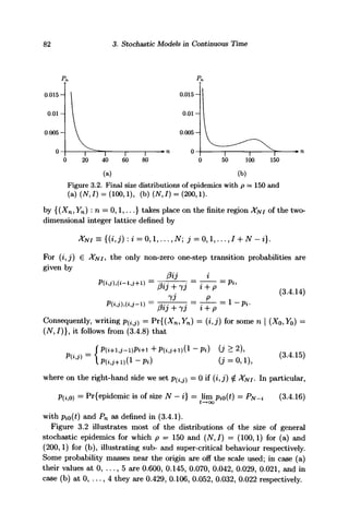
Figure 3.3. Conditional mean durations of epidemics with p = 150 and
(a) (N,I) = (100,1), (b) (N,I) = (200,1). Abscissae give the number of
susceptibles infected. The means were not computed for large n for which
Pn = pjy-n.o < 10~9
. Cf. Exercise 3.13 and Daley et al. (1999).
We have also computed the conditional mean durations of these epidemics
with /? = 1 for those final sizes for which the probabilities exceed 10~9
. In
the notation of (3.4.12), we have found ri0 = T(N,i),(i,o) for those i for which
P(i,o) > 10~9
. These conditional means satisfy the recurrence relations, for
{i, j) € XNI, starting from r^v/ = 0,
U >
and
where fiij = l/[j(p + i)] = 1/q^j) for the state (i,j) in the notation of
(3.4.13). They are illustrated in Figure 3.3 for the same two epidemics as
in the previous figure.
3.4.4 Behaviour of the general stochastic epidemic model: a
composite picture
We now draw together these and other results to describe in general terms
how the general stochastic epidemic model behaves, and point out some of
its weaknesses.
First the Threshold Theorem distinguishes between sub- and super-crit-
ical conditions. In the case of a sub-critical epidemic, the numbers of infec-
tives and removals behave roughly like live and dead individuals in a sub-
critical birth-and-death process. This is borne out principally by Whittle's

96. 84 3. Stochastic Models in Continuous Time
Threshold Theorem 3.1. Both the duration and final size of the epidemic
process are roughly the same as for the approximating birth-and-death pro-
cess.
The super-critical case is more involved. Here it is possible that only a
minor epidemic occurs, with probability approximately (p/N)1
. The size of
such a minor outbreak is similar to that of a super-critical birth-and-death
process conditional on extinction. Prom the work of Waugh (1958), this
is exactly that of a sub-critical birth-and-death process whose linear birth
(death) rates are the linear death (birth) rates of the original super-critical
process respectively. Otherwise, the early behaviour of the epidemic pro-
cess is similar to that of a super-critical birth-and-death process conditional
on non-extinction, until the number of infectives represents an apprecia-
ble proportion of the initial number of susceptibles. If the deterministic
model of the epidemic is any guide, the evolution of the epidemic process
through a number of generations of infectives is still similar to the birth-and-
death process (see Figures 2.7 and 2.8 and Exercise 3.5), until the number
of susceptibles approaches the borderline value p between sub- and super-
criticality. At this stage, in terms of numbers of susceptibles and infectives,
the process follows approximately the solution of the deterministic epidemic
model (with E X(t) « x(t) etc., much as for the simple epidemic; cf. Exercise
3.1). The 'imprecision' of the approximation, which in model terms incor-
porates both the stochastic lag and variability about the mean behaviour
(~ deterministic solution), is approximately normally distributed if N and
p < N are both sufficiently large. This leads (Barbour, 1972, 1974) to the
ultimate number of susceptibles being approximately normally distributed
about the mean EX(oo) « NO, where NO is the number of susceptibles
surviving the deterministic epidemic, with a variance that can be computed
using Kendall's 'Principle of Diffusion of Arbitrary Constants' (cf. Daley
and Kendall, 1965, and Section 5.4 below).
If it happens that Ro = N/p is somewhat larger than 1 (e.g. 3 or more),
then, conditional on the occurrence of a major outbreak, the number of
susceptibles surviving the epidemic is approximately Poisson distributed,
still with mean NO where 0 is now much closer to 0 (cf. Daniels, 1967).
This number can be regarded as representing those individuals having a
'small' chance of avoiding infection. If NO is itself not close to 0, then the
closeness of a Poisson distribution to normality ties together this result with
the previous paragraph. Sellke (1983) proved Daniels's result by considering
a sequence of general epidemic models with parameters (Nk, Ik, pk). These
parameters are such that as k —> oo, all three diverge to oo in such a way that

97. 3.5. The general stochastic epidemic in a stratified population 85
—> M, say, for some finite positive M. Then the number of
susceptibles Xfc(oo) ultimately surviving the epidemic is shown to converge
in distribution to the Poisson with mean M.
This ultimate size distribution is considered in more detail for the different
cases of N and p in Nagaev and Startsev (1970) (see also Nagaev, 1971)
using the embedded jump chain. The most general formulation of such
results may be found in Reinert (1995).
In the limit theorem setting for these results, the duration of the epidemic
may ultimately be exceedingly short; this indicates a need for rescaling time
or else reviewing the conditions under which the model may apply. When
one considers the observation of measles epidemics in large cities as reviewed
in detail by Bartlett (1960), it becomes clear that the time- and generation-
dependent evolution of the models need modification if they are to reflect
this aspect more realistically. Fortunately, both the stratification models of
the next section, and the chain binomial models of the next chapter, offer
avenues for overcoming the drawbacks of the overly simple S-I-R model.
3.5 The general stochastic epidemic in a stratified population
This section starts by describing a continuous time Markov process model
that extends the ideas of Section 3.3 to a stratified population, consistent
with the deterministic setting of Section 2.4. In that setting we discussed
what criterion should be used to distinguish a major from a minor out-
break; in the stochastic setting two further factors need to be considered,
namely the discreteness of the population, and the stochastic modelling of
the infection and removal processes. These factors lead us to a digression
on the notion of the Basic Reproduction Ratio of an epidemic model. We
conchide the section with an example of a stochastic model for an epidemic
taking place in a community of households, a problem to which we return
in Chapter 7.
A stochastic analogue5
of the general deterministic epidemic of Section
2.4 assumes that a finite population of susceptibles is stratified into m
groups of sizes N = (TV^,..., ATm)', where as in Section 2.4, vector nota-
tion is convenient. At time t — 0 suppose a single infective is added to
5
Daley and Kendall (1965) remark that the 'natural' formulation of a population
process at the micro-level is discrete and (more than likely) stochastic. From this point
of view, a discrete stochastic model is the prototype of which the deterministic model,
with both continuous state space and deterministic (non-stochastic) evolution, is the
analogue or approximation. As Barbour (1994) puts it, a deterministic model 'only has
a meaning as an approximation to some underlying jump process'. Anderson and May
(1991) consider deterministic models almost exclusively.

98. 86 3. Stochastic Models in Continuous Time
stratum i. At time t > 0 the jth group consists of Xj(t) susceptibles,
Yj(t) infectives and Zj(t) = Nj + 6ij - Xj(t) - Yj(t) removals, so that
{Xj.Yj.Zj^O) = (Nj.Sij.O), (j = l,...,m), with 6{j the Kronecker delta.
We use a continuous time Markov process to model the infection and re-
moval mechanisms, analogous to that used earlier in this Chapter. As in
Section 2.4, faj denotes the pairwise rate for an infective in i to infect a sus-
ceptible in j , and jj the removal rate per infective in j . In vector notation,
the property of constant sizes of the several strata is expressible as
X(t) + Y(t) + Z(t) = N + U (all t), (3.5.1)
and the initial condition is that (X, Y, Z)(0) = (N, li, 0), where the m-row
vector li has 1 as its i th component and all other elements zero.
The process {(X,Y, Z)(£) : t > 0} takes place on a finite state space,
so it is completely specified as a continuous time Markov process when its
initial state and infinitesimal transition probabilities are given. We know
(X,Y, Z)(0) already, and the constraint (3.5.1) means that it is enough to
describe (X, Y)(t). We assume that for the strata i = 1,..., ra, with x and
y denoting m-vectors of non-negative integer-valued components,
<5*) = ( x - l i > y + 1,-) | (
= *i(££iAj!fc)« + o(6t) - Xj(y'B);«t 4- o(St) {x3 > 1),
Pr{(X,Y)(t + ft) = ( x , y - 1,-) | (X, Y)(t) = (x,y)}
= *yjyj6t + o(St) {yj > 1),
Pr{(X,Y)(t + ft) = (x,y) | (X,Y)(t) = (x,
(3.5.2)
where B = (Aj)- We can now write down the forward Kolmogorov equa-
tions, but they are too unwieldy to give an explicit solution, whether in
the time or transform domain. We have described this model here because
(a) it is easily studied via simulation techniques, (b) it is general enough to
capture inhomogeneity, and (c) it provides an adequate setting to discuss
the basic threshold phenomenon.
We first consider a method of approximating the behaviour of the process,
entirely consistent with Whittle's approach in Section 3.2. This approach
effectively keeps the size of the susceptible population fixed during the early
stage of the epidemic, so that the only changes occurring in the population
are in the numbers of infectives Y say. In the m-strata context we there-
fore approximate the process by a multi-type linear birth-and-death process

99. 3.5. The general stochastic epidemic in a stratified population 87
), in which at time t there are Yj(t) (j = I,..., ra) j-type individuals, for
whom the birth and death rates are respectively YALI 0ijYi(t)Nj anc
* lj%
provided no Nj is small these birth rates differ little from YllLi Aj^i W^O W
for t small enough (cf. (3.5.2)). This process Y(t) is an irreducible multi-
type Markovian branching process in continuous time. For such processes
it is known (e.g. Athreya and Ney, 1972, §V.7.5) that the vector q whose
i th element
qi = Pr{ lim ^ ( t ) = 0 | Y(0) = 1*} (3.5.3)
gives the probability of ultimate extinction, is the least positive solution of
the equations
YfjLiPtjNjqiqj + 7i = QL'jLiPijNj + li)Qi (i = 1,..., ra). (3.5.4)
Now qi = 1 (all i) is always a solution, but need not be the least positive
one. Also, the process is irreducible if and only if the matrix B is primitive,
meaning that for some integer n, which is at most equal to ra, B n
has its
(z,j)th element positive. Because of irreducibility, either <ft < 1 (all i) or
else qi = 1 (all i), and the former holds if and only if
B diag(N) - diag(7) (3.5.5)
has a real positive eigenvalue; this is equivalent (see Exercise 3.9) to R > 1
where R is the largest eigenvalue of the non-negative matrix
Mi = diag(7~1
)Bdiag(N). (3.5.6)
In the one-dimensional case equation (3.5.6) gives R = f3N/j = N/p =
RQ, and the condition R > 1 is exactly the condition in Whittle's Threshold
Theorem 3.1 for a major outbreak. Thus, we have indeed generalized that
result to the ra-strata context.
For birth-and-death processes, as for branching processes and random
walks, conditions for behaviour like extinction or return to the origin, are
typically given both probabilistically and in terms of first moments. Ap-
plication of the latter method to epidemics makes use of the Basic Repro-
duction Ratio. This is defined for epidemics in homogeneous populations
as 'the average number of persons directly infected by an infectious case
during its entire infectious period, after entering a totally susceptible pop-
ulation' (Giesecke, 1994, p. 111). This definition formalizes the notion that
a major epidemic will occur when, in the earlier stages of an outbreak of a
disease, each infective on average produces more than one further infective.

100. 3. Stochastic Models in Continuous Time
In particular, in the simplest case (/ = 1) of the general epidemic model
of Section 3.2, the initial infective is placed in a population of N suscep-
tibles where it mixes homogeneously during its infectious period T, with
T exponentially distributed with mean I/7. Then the number among the
N initial susceptibles contacted (and therefore, potentially infected), is a
binomial r.v. Bin(iV, 1 — e-/3T
). Unconditionally therefore, if susceptibles
are affected only by the initial infective until its removal, the mean number
of new infectives directly contacted by the initial infective equals
* ^ ,3.5.7)
P
where i^o is as below (3.5.6), and the approximation is valid when p ^> 1,
i.e. (3 <C 7. While this condition is stated in terms of p rather than TV, the
case of super-criticality (i.e. RQ > 1) then implies that N ^$> I. The analogy
of the criticality condition, that Ro < or > 1, with that for Galton-Watson
branching processes, is immediate.
To apply this idea to the m-strata context, we refer to the initial infective,
in stratum i say, as a zero generation z-stratum infective. Let m^ denote
the expected numbers of first generation j-stratum infectives (j = 1,..., m)
to which it gives rise. We ask whether these various first generation in-
fectives in different strata, if each is placed in the same environment of N
susceptibles as the initial infective, would produce on average a larger num-
ber of second generation infectives, and so on. Now the expected number
of /c-stratum second generation infectives produced by an initial i-stratum
infective, on the assumption that each first generation infective is placed in
the same initial population of N susceptibles, equals Y^JjLi rriijmjk, i.e. the
(i,/c)th component of the matrix M2
where M = (rriij). Continuing this
process, the expected numbers of j-stratum infectives after r generations,
for r not too large, equals the (i,j)th element of the matrix Mr
. Since
M is a non-negative matrix (indeed, it is primitive because B is primi-
tive) , Perron-Frobenius theory implies that each column of Mr
is like RQV
for large r, where Ro is the largest eigenvalue of M and v is the right-
eigenvector corresponding to Ro. It follows that the expected number of
infectives after r generations either dies away to 0 when RQ < 1, or else
grows exponentially for a while when RQ > 1, reflecting the possibility of a
major outbreak.
To identify M, note that an i-stratum infective is infectious for an expo-
nentially distributed time Ti with mean 1/7^ If the N susceptibles were not
otherwise subject to infection during this period T^, the number of j-stratum

101. 3.5. The general stochastic epidemic in a stratified population 89
infectives produced would be a binomial r.v. Bin(iVj, 1 — e~^T%
). Hence,
unconditionally, the expected number m^ of first generation j-stratum in-
fectives produced by an z-stratum infective is given by
mil - m i - .-*.«) = NS(1 - ^ - ) - M4 , (3.5.8)
the approximation again being valid for 0ij <C 7*. The matrix M is
M = (f^) « ( ^ ) = diag(7-1
)Bdiag(N) = Mlt (3.5.9)
with Mi as at (3.5.6). It follows that RQ « R, and we should call RQ the
Basic Reproduction Ratio for the epidemic. This terminology is that of
Diekmann, Heesterbeek and Metz (1990) who noted that it is a dimension-
less quantity (hence, ratio rather than rate or number), which measures
'reproductiveness'. The discussion concerning Examples 3.5.1-2 supports
our contention that this moment-based definition for Ro is more appropriate
than R, defined in more probabilistic terms around (3.5.6). We summarize
our discussion thus far.
Theorem 3.2. A stochastic epidemic in a stratified population such that
no component of N is small, with infection rates faj and removal rates
jj as for (3.5.2), exhibits sub- or super-critical behaviour (i.e. only minor
outbreaks occur, or major outbreaks may occur) according as the Basic
Reproduction Ratio RQ is < or > 1, where RQ is the eigenvalue of largest
modulus of M = (m^).
The birth-and-death continuous time approximation, leading to Mi, and
the generation-wise approach leading to M, give similar but not exactly
identical conditions for distinguishing between sub- and super-criticality.
Under the first approach the matrix Mi is computed after a single jump
of the process whereas contributions to the matrix M arise from both this
single jump and possibly several subsequent jumps. Because of this, ap-
proximations based on M are better than those based on Mi.
Stochastic analysis of the model defined by (3.5.2), such as the computa-
tion of the ultimate size of an epidemic, is complicated by the dimensionality
of the state space needed to provide a Markovian description of the process.
Clearly, one possible description is the (2m)-dimensional process (X, Y)(t).
If the size of m is appreciable, this may be too large for exact computation.
When the parameters fiij and 7 have a simple structure, the analysis can
be correspondingly simplified, as in the following Examples.

102. 90 3. Stochastic Models in Continuous Time
Example 3.5.1 (m interacting communities). Consider a population which
consists of m communities of Ni individuals (i = 1,..., ra), all of whom are
susceptible to a disease which, if introduced, spreads by pairwise contact at
rates (3u = (3H (all i) and fa = (3C (all (z, j) with i ^ j), where (3H > /3C
(typically, @H ^ Pc)- Removal of infectives occurs at a common rate 7
per infective. Suppose that a single infective is introduced into the ith
community. Using the approximations at (3.5.9), the Basic Reproduction
Ratio that gives us a threshold criterion is the largest eigenvalue of the
m x m matrix Mi with elements
Thus, #0 is the largest positive root of the characteristic equation /(A) = 0
where
/(A) = det
f}HN2h-
= det
with Nj =
/(A) =
0
0
(3HCN2-
0
X 0 0 ...
and /3Hc = PH — Pc- Expanding the determinant,
i=2
- A) J(0HcNi - A) + /3CN2(/3HCNI ~ A) HiPncNi - A)
i=3
m-1
+ • • • + PcNm(f3HCNi - A) FJ (J3HCNi - A)
i - A)) P
+
This expression is a polynomial of degree m in A; we require the largest A
solving /(A) = 0. By inspection we see that the m-fold product is finite

103. 3.5. The general stochastic epidemic in a stratified population 91
and non-zero for A > max; PncNi, SO any zero of the second factor in that
region is a candidate for Ro. Now this second factor is strictly increasing in
A for max* 0nc^% < A < OO, ranging from —oo at the left-hand end of this
semi-infinite interval to -f1 at -foo, so
y ( )
fe i - X
has exactly one zero there. Therefore Ro equals this zero, i.e.
Ro> {3HCmaxNi. (3.5.13)
i
Each term on the right-hand side of (3.5.13) is increasing and convex in
so by Jensen's inequality
mfoAT/jr
-RfaN/j' K
'
where N = Y1T= N»/ra; equality holds if and only if either 0H = Pc or
Ni = Nx (all i). Hence, when 7 > (3H > (3c,
Ro > PH + (m - )PcWh, (3.5.15)
with equality holding as for (3.5.14).
When the fiij and 7^ have the structure of this Example but without
the condition 7 » max(f3ci PH), the approximation given in (3.5.8) should
not be used. In place of /(A) = det(Mi — A/), we must instead identify
Ro with the largest root of det(M — XI) = 0. Exercise 3.10 details the
changes to (3.5.13-15) that then ensue. For example, if /?# = 1 = 7,
/3c = 0.001, m = 101 and all JVj = N, (3.5.15) used as an approximation
gives Ro « 1.1Ni whereas the analysis in Exercise 3.10 gives Ro = 0.60(Wi.
We also emphasize that the discussion and example above are based on the
assumption that all components Nj of N are 'large'. To illustrate what may
happen when this assumption is false, suppose that (3H — 100, 0c — 0.0001,
and the other parameters are those just considered. Using Exercise 3.10
yields Ro ~ l.OOOliVi, which we interpret as N new infectives within the
household containing the initial infective, with only a small expected num-
ber of infectives in other households. Because the household sizes are small,
the disease must be propagated outside the household of the initial infec-
tive for a major outbreak to occur. The expected number of such outside

104. 92 3. Stochastic Models in Continuous Time
contacts is at most about O.OlJVi per infective per generation, as against
about iVi infectives produced within the household of any such infective.
So in two generations there may be up to about O.OlATf outside infectives
produced per initial infective, corresponding to O.liVi new infectives per
generation. Consequently, until N is about 10 or more, no major outbreak
can be expected (see also Exercise 3.11), contrary to the interpretation that
follows from Theorem 3.2 when Ro > 1 which holds for all JV~i > 2. This
contradiction stems from assuming that all Nj are large. Fortunately we
can rework the analysis on the basis of distinguishing newly infected in-
dividuals, not by the stratum or household to which they belong, but by
the number of susceptible individuals in the same household who remain
susceptible after the initial infective is removed, before the influence of any
secondary infectives.
Example 3.5.2 (A community of m households). Assume the model of
the previous example, where the strata are now households. Suppose a
given infective is initially in a household with i susceptibles, and call it an
z-type infective. Assume that the initial infective is infectious for a time T,
and that during this infectious period, only the initial infective can make
susceptibles infectious. At the end of this infectious period, identify each of
the individuals now infected by the number j of susceptibles remaining in its
household. Then the probability that j susceptibles remain in the household
of the initial infective at the end of the random time T is PijiPn), where
( 3 5 1 6 )
(see Exercise 3.11). For any other household where there are initially i
susceptibles, the probability that j susceptibles remain after the random
time T is Pij((3c)- Regard the household of the initial infective as being
additional to the initial population of N susceptibles as described; then the
expected number rrtij of j-type infectives produced by this initial i-type
infective is given by
(3.5.17)
r=l
say. Define M = (m^). Then using the same argument as above (3.5.8),
the expected number of second generation fc-type infectives (i.e. infectives
in households with k susceptibles) equals the (i,/c)th element of M2
. We

105. 3.5. The general stochastic epidemic in a stratified population 93
conclude that, with n' = maxi<r<m(7Vr — 1), the Basic Reproduction Ratio
.Ro for the process is the largest eigenvalue of the (p! + 1) x (n' + 1) matrix
M =
^H
m0 m
mi
i +mi
... mn'
VTL2
^ / o ( ^ i ^ 2
(3.5.18)
Explicit computation of this eigenvalue does not appear possible in general.
We can compute the limiting value of Ro when /3H ^> 7 because then
p^ ^ fijo a n
d i?o is the largest root of /C(A) = 0, where
/c(A) = det
mo — A
1 + 7Tio
2 + mo
m i vri2
i — A rri2
mi m2 — A
= det
r
mo — A mi rri2 - •. rnn>
1 + A - A 0 ... 0
2 + A 0 - A ... 0
in' - A
n' 0 0 ... - A J
say.
Thus, when /?# ^> 7,
The expressions for A and f? implied by (3.5.19) reduce to
A =
because
' + 0c '
A =
(3.5.19)
(3.5.20)
(3.5.21)
where terms in the inner summation are zero for j > ATj, and the inner
sum equals the expected number of infectives in a given household of iV»

106. 94 3. Stochastic Models in Continuous Time
susceptibles produced by a single infective outside the household. Introduce
Ni identically distributed indicator r.v.s Ik (k = 1,..., Ni) to denote that
the kth susceptible in the household is infected. Then EIk is just the
probability that this kth individual is infected before the initial infective
becomes a removal, so Elk = /?c/(7 +A?)» and the expression for A follows.
Similarly,
in which the inner sum is expressible in terms of the same indicator r.v.s as
E
where k ^ k1
. Using properties of exponential r.v.s, we see that E(Ik'Ik) =
2/?c£c/[(7+2/?c)(7+/3c)]. Collecting terms together then leads to (3.5.21).
To illustrate the relevance of the assumption that (3H ^> 7, suppose that
/3H = 1 = 7, /3C = 0.001, m = 100, TV* = Nx = 3 (cf. the example in the
text below (3.5.15) where we should have Ro — 1.8 from Exercise 3.10).
Then from (3.5.18), det(M — XI) — 0 is a cubic equation, with largest
root RQ = 0.7864, whereas the approximation at (3.5.20) which depends on
0H ^> 7, gives J^o ~ 0.9369. The same approximate Ro holds on changing
/3H to 3, but the corresponding exact root 0.8992 is closer to it, and closer
still (Ro = 0.9318) for (3H = 9. See Ball, Mollison and Scalia-Tomba (1997)
for related work.
3.6 The carrier-borne epidemic
Suppose that a population of X(t) susceptibles of initial size n is being
infected by W(t) carriers of a disease with W(0) = b, who are themselves
immune to infection but subject to a pure death process. Any infected
susceptible is directly removed from the population. Then the stochastic
process X(t) is subject to the influence of the process W(i) which is inde-
pendent of X(t).
Let the death process {W(t) : t > 0} be a homogeneous Markov chain in
continuous time with death rate 7; then we know that its p.g.f. is
(ye'* + 1 - e"^)6
(v < 1), (3.6.1)

107. 3.6. The carrier-borne epidemic 95
so that
Pr{W(t) =fc| W(0) = b} =
and
E[W(t) | W(0) = b) = fcT7
* - tu(t)
where iu(£) is as in the deterministic carrier model of Section 2.6.
To analyse the process {X(t) : t > 0}, assume that {(X, W)(t) : t > 0} is
a bivariate Markov chain with transition probabilities
Pr{(X, W)(* + St) = (i - 1, fc) | (X, W){i) = (i, fc)} = /3ifc6t 4-
= (t,fc- 1) | (X, W)(t) = (i, fc)} = jh6t + o(6t),
= (i, fc) | (X, W)(«) = (t, fc)} = 1 - (/?* + 7)* «* - o{6t).
The forward Kolmogorov equations for the process are given for 0 < i < n,
0 < fc < 6, by
= P(i + l)fcpi+i,fc - ()
dc
subject to the initial condition pn6(0) = 1, where
Pik(t) = Pi{(X,W)(t) = (i,k) I (X,W){0) = (n,b)},
and pn+i,fc = Pi,b+i = 0 when either i or fc lies outside its respective range.
Use the same transformation tf
= (3t as at (3.2.2), and set p = j/(3. Then
for 0 < i < n, 0 < fc < 6, the forward Kolmogorov equations become
jj^ i|fc - (t + p)fcpifc + p(fc + lKfc+i (3.6.2)
with the initial condition pnb(fy =
1- For convenience, we use t below for
this new t1
.
We discuss two methods for solving this equation: the first is the p.g.f.
method discussed earlier, while the second is based on a method of Puri
(1975) for a Markov process developing under the influence of another pro-
cess. Such a process could be described as a doubly stochastic Markov
process by analogy with the previously named doubly stochastic Poisson
process.

108. 96 3. Stochastic Models in Continuous Time
Referring to (3.6.2) we derive for the p.g.f.
, v, t) = E ( / W ^ W ) = Yl PikWzW (0<z,v< 1),
0<i<n,0<k<b
the p.d.e.
subject to the initial condition (p(z,v,Q) = zn
v6
.
To solve this equation, assume that ip{z,v,t) = Z(z)V(v)T(t) and use
the standard method of separation of variables. Then from (3.6.3) we have,
writing f = dT/dt, Z' = dZ/dz and V =
t Z1
V V
so that T = e~xt
directly. We also see that
Z _ P ( l - 1 ; ) A V _
11 Z)
~Z~ v W'~~h ( j
where j is a quantity that we discuss shortly. These relations lead to
&___Z3_ V _ A
so that, apart from constants,
V
-(-r
Now we know that </?(z, v, f) must be a polynomial in z and v, of degree
n in z and 6 in v. Hence j must be an integer in the range 0 < j < n, and
so too must 0 < X/(j + p) < b. Corresponding to a particular value of j ,
the eigenvalue A^ will be
It follows that
n b
Y^'^/C', t/, LJ — 7 7 L-jf^Kj yL — Zl I C — ~ I , I O.D.U)

109. 3.6. The carrier-borne epidemic 97
where we now need to find the values of the coefficients Cjk- We do this by
setting t = 0, when
<p{z,v,0) = zn
vb
=
j=0 fe=
Writing £ = 1 — z, 77 = 1; — p/(j + p), this reduces to
j=0 fc=0
whence Cj^, being the coefficient of £J
7/fc
in the expansion of the left-hand
side, can be identified as
and
It is easily checked that for z = 1 we recover y?(l, v, t) = [l -f- (v — l)e~pt
] ,
i.e. the p.g.f. (3.4.1) of the pure death process W(t), following the change
in time parameter at (3.2.2).
The joint distribution of (X, W)(t) for any t > 0 can be found by expand-
ing (3.6.8). Perhaps more important is the distribution of X(t) whose p.g.f.
equals
(3.6.9)
It follows that
= i | X(0) = n} =
C::)[%]

110. 98 3. Stochastic Models in Continuous Time
and
For the deterministic model of Section 2.6 the analogous function is x(t),
given at (2.5.4). Rewrite it, after changing the time-parameter to make it
consistent with the notation used in this section, as
x(t) = n exp ( —
Then
l l t T I T * i / l TDf* I r ^
11x11 JUV I — ILKZ
t—• OO
where the inequality, a trivial consequence of ely/p
> 1 + 1/p, shows that
the expected ultimate size of the stochastic epidemic is smaller than the
ultimate size of the deterministic epidemic. More precisely, we can show
that lim^oo (E[X(£)] - x(t)]) « 6/2p2
, which is o(l) for small to moderate
integers b and somewhat larger integers p. See Exercise 3.12 for more detail.
As in the case of earlier models, we are interested in the number of initial
susceptibles that are ultimately infected. For this, we can readily obtain
the probabilities P^ = imt-^oo Pn-k,•(£)of the size k of the epidemic from
(3.6.10), namely
= (I)B-1
)^
Let T be the duration of the epidemic and F its d.f. Then F(t) =
Pr{no further infection after t} is given by
F(t)=Po.(t)+p.o(t)-Poo(t),
where the terms on the right-hand side can be determined algebraically from
(3.6.10), (3.6.1) and (3.6.8), respectively. Hence,
(3.6.13)

111. 3.6. The carrier-borne epidemic 99
In the particular case 6 = 1 this expression simplifies and yields for example
E(r | vr(0) =U =j f [i-"Ml<•«=J - 1 (j) £ f
P Jo P Jo
(Bailey, 1975, p. 196). For integers b > 2, the complete beta integral here
is replaced by one or more incomplete beta integrals that can no longer be
simplified.
The following, alternative approach, due to Puri (1975), relies on the
observation that, conditional on W(-)> ^ W 1S
itself a pure death process
with the random, time-varying death-rate parameter j3W{-). This implies
(e.g. Kendall, 1948) that
{W(u) :0<u<t}) = (ze~W
^ + 1 - e -^*>)n
, (3.6.14)
where W(t) = /0* W(u)du, the initial condition (X,W)(0) = (n,6) being
understood. Expanding (3.6.14) and taking expectations yields the p.g.f.
(3.6.15)
The problem now is to evaluate the expectations on the right-hand side.
This can be done^via the joint Laplace transform of the bivariate Markovian
process (W(t),W(t)),
fl{v, 0, t) = E(vw
We-^W) (M < 1, Re(6) > 0),
for which the corresponding probability terms are
qbk(u, t) = Pr{W(t) - jfe, W(t) < u | W(0) = b}.
The forward Kolmogorov equations for these functions q^ are easily derived
because {W(i) : t > 0} is a pure death process: we find

112. 100 3. Stochastic Models in Continuous Time
with qkk(u,0) = 1 (all u > 0). Now
subject to n(v, 0,0) = f6
. Taking Laplace transforms, equations (3.6.16)
become
1 an an _ p an p an
0 at"+v
a^ ~~" 0v
& 7 +
^
or
f = K« + P)«-P]f • (3-6.17)
This equation can be solved by using Lagrange's method: write
dt dv d0 dA
T ~ {0 + p)v-p ~ T ~ 0 '
whence
In ((0 + v)p - p) = (0 + p)t -f A, ft = B,
where A and i? are constants. It follows that
ft(t;, e, t) = f{e-(e+
^{{9 + p)v - p]), (3.6.18)
subject to fl(v, 9,0) = vb
, i.e. vb
= f([$ + p]v - p), so
This gives
f ( ^ p{1
-;-{e+P)t)
)b
(3.6.19)
o + P
Setting 0 = j for j = 0,..., n and combining the resulting expressions as in
(3.6.15), we recover (3.6.8).
Other examples exploiting this method can be found in Puri (1975).
3.7 Exercises and Complements to Chapter 3
3.1 The analogue of t3 at (3.1.3) in the deterministic simple epidemic is the
solution t'3 of the equation (cf. (2.1.2)) x{t'j) = j — 1, equivalently, y(t'j) —
N + I + l-j. Show that
, 1 . N(N + / + 1 - j)
3
/3(N + I)m
I(j-l)

113. 3.7. Exercises and Complements to Chapter 3 101
and hence deduce that when / > 2,
where JN,I,J is defined below (3.1.4). This quantity is negative, and is some-
times called the stochastic lag. An alternative derivation entails the use of
the approximation ]T^_ i~l
~ / _i^ u
~l
^u
-
3.2 Show that in the special case of a simple stochastic epidemic starting with
one infective introduced into a population of N susceptibles, the first two
moments Eii and varti of the duration t of the process in Section 3.1 are
related by
1 An 1 i»_ 2/?E«x +ig2
+O(JV-1
)
1
/32
(N + 1)2
^ [ i N + l
Observe that varti/(E*i)2
= [l/(iVlniV)](l + o(l)) for large AT.
3.3 (a) Check that for real s, the gamma function
/
OO /»OO
e-y
y~ts
dy = / e1M
J -OO
exp(-a: -
is the characteristic function of the extreme value distribution with p.d.f.
exp(—x — e~x
). Hence deduce that the asymptotic distribution of W at
(3.1.18), having for its Laplace-Stieltjes transform the product of two gamma
functions, is the convolution of two extreme value density functions:
/•oo
(W,W + dw)} = / exp(-v - e'v
) exp[-(w - v) - e"^'^] dv dw,
J —oo
which reduces to the density at (3.1.21) (Kendall, 1957).
(b) To explain why the extreme value distribution occurs in the limit distri-
bution for the duration t of the simple stochastic epidemic of Section 3.1,
take N even, N = 2M say, with 1 = 1 and show that t is expressible as
the sum Ui + U2 of i.i.d. r.v.s Uk =d X ^ i Si/[i(2M + l-t)](lb = 1,2),
where Si, ft,., are i.i.d. unit exponential r.v.s. Deduce that each Uk lies
between U'/M and U'/(2M), where U' is the r.v. U' = Y™ =1 Si/i. Show
that U' =d maxi^if^}, and that (M + )Uk - lnM and (M + l)U' - lnM
both converge weakly to the same limit r.v. with the extreme value density
of (a). (See Kendall's paper for details.)

114. 102 3. Stochastic Models in Continuous Time
3.4 (See also Example 3.3.1.) For the general stochastic epidemic model of Sec-
tion 3.3 starting from (N, I) = (1,1), and assuming that 0^% 27, use direct
d.e. solution methods to solve the equations p n = -(/3 + 7)pn, pio = 7Pn>
p02 = pPll - 27/?o2, Poi = 27P02 - 7Poi, Poo = JPoi- For example, show that
7(1 - e ^ ^ ) p ,F2 /*T
3.5 (Cf. Section 3.3.2 and Figure 2.4.) In a linear birth-and-death process {Y(t) :
t > 0} with birth and death rates A and fi per individual, where X > fi
and Y(0) — / , suppose that at time t there are Y3(t) jth generation live
descendants of the original / individuals and Zj (t) j th generation descen-
dants no longer living (cf. Section 2.5). Show that the expected numbers
yj(t) = EYj(t) and Zj(t) = EZj(t) satisfy the system of d.e.s
yj=yJ-i- HVJ, ZJ=MJ 0 = 0 , 1 , . . . ) ,
provided we set y-i(t) = 0. Deduce the solution
J- o
so that m(t), the 'average' generation number of the {z3(t)}, is given by (cf.
Figure 2.4)
u Xt X
Waugh (1958) proved that a super-critical linear birth-and-death process
conditional on ultimate extinction, behaves like the birth-and-death process
with birth and death rates interchanged, and so is sub-critical. Use this result
to show that
jZ,(u) | H I ) - 0 (I - oo» =
Deduce that Pr{Y(t) —•0} = (^/A)7
, so that for the non-extinction set
{Y(t) -+ ex)}, setting r = /i/A,
E[^.jZ3(u)Y(t) -^ 00 (t ^ 00)}
A [(A - fi)u - l][e(A
~^u
- r7
e-( A
-^) u
] + 1 - r1
A — X e(*-»)u _ rI-le-(-n)u _ I + rI-l

115. 3.7. Exercises and Complements to Chapter 3 103
3.6 For the general stochastic epidemic, show that the first passage time distri-
bution into any state can be constructed as a weighted sum of convolutions of
distributions of exponential r.v.s, where the components of the convolutions
correspond to the sojourn times in the states visited along the paths and the
weights are the respective probabilities of those paths.
[Remark. The same result holds true for any continuous time Markov pro-
cess on countable state space with well-ordered sample paths and bounded
transition rates. This algorithmic principle explains why the p.g.f. method
is applicable to the simple and general stochastic epidemic models.]
3.7 Show that if j is a non-absorbing state in a Markov process with well-ordered
sample paths, then -K%3 = q3 /0°° Pr{X(u) = j X(0) = i}du (cf. (3.4.8)). In
particular, for the general stochastic epidemic as in Section 3.4.3,
Pi*,,) = W8 + 7W / Pr{(X,y)(t) = (ij) | (X,Y)(0) = (N,I)}dt.
Jo
[Remark. This principle, complementary to the previous exercise, underlies
the simplicity of the jump-chain algorithm for computing both intermediate
and final state probabilities of strictly evolutionary Markov chain models.]
3.8 Using the same notation as at (3.4.10), show that the quantities
T™ = E(t2
ik | X(0) = i,X(u) = k for some u > 0),
starting from rit = 0, satisfy the recurrence relation
=
3.9 Let the m x m non-negative matrix A be primitive, and let the diagonal
matrix D have all elements positive, much as in Section 2.4. Use Perron-
Frobenius theory (e.g. Seneta, 1981, Chapter 1) as at Lemma 2 of Daley and
Gani (1994) to show that
(i) the eigenvalue Amax of A — D that has largest real part, is real;
(ii) the eigenvalue /imax of AD'1
that has largest modulus, is real and posi-
tive;
(iii) Amax <, = or > 0 according as /imax <, = or > 1, respectively.
Suppose that the pairwise infectious rates fiio of Sections 2.4 and 3.5 have the
product form 0i3 = frcty so that B = (0%3) = 0a where the vectors 0 and
a have components /3t denoting the infectivity rate of infectives in stratum i
and relative susceptibility of susceptibles in stratum j . Show that when Mi
at (3.5.6) is primitive, its largest eigenvalue is R = ^2iNlat/3t/ji. When is
it true that R w RQ, the Basic Reproduction Ratio for such an epidemic?

116. 104 3. Stochastic Models in Continuous Time
3.10 In the context of Example 3.5.1, with the 0tJ as given there, show that the
dominant eigenvalue ifoofthemxm matrix M of (3.5.8), is as at (3.5.12)
if we replace Nt by Nx, 0Hc by 0H/(0H + 7) - 0c/(0c + 7) a n d
0c by
0c/(0c + 7). Deduce that when N3 = Ni (j = 2,... ,ra) (cf. (3.5.13)),
_ {[(m - l)/
Check that this is smaller than the case of equality in (3.5.15), which ap-
proximates this expression if 7 ^> max(fc,fe).
3.11 Derive (3.5.16) using the embedded jump technique of Section 3.4.2. Show
that when 0 < 7, PtJ(0) « (0h)%
~3
(i/j)> Use (3.5.20) to conclude that in
the setting of Example 3.5.2, RQ > 1 when N% > l/(ra/fc/7); this condition
yields N > 4 when m = 100 and 0C = O.OOI7, and Ni > 10 when m = 100
and /3c = O.OOOI7 (cf. the text preceding Example 3.5.2).
3.12 Use the generating function (3.6.8) to show that for the stochastic carrier
epidemic,
r 1 - U
E[X(t)W(t)} = E[X(t)} E[W(t)]e-* [l
1 + p
and deduce that cov(X(t),W(t)) < 0 for 0 < t < oo. Use (3.6.11) to
conclude that (d/dt)E[X(t)} = -E[X(t) W(t)] > -E[X(t)]E[W(t)]. Hence,
since E|W(£)] = w(t) (see below (3.6.1)), conclude that for the deterministic
and stochastic carrier models, the inequality
±(x(t) - E[X(t)]) < (x(t) - E[X(t)])w(t)
is satisfied. Since (X, VF)(0) = (x,ii;)(0), the right-hand side is zero at t = 0
and thus is negative for all sufficiently small positive t, hence negative for all
finite positive t, and therefore
0 < E[X(t)] - x(t) T n[(l + p"1
)"6
- e~b/p
} (0 < t T oo).
[Remark. Alternatively, differentiation shows that when 6 = 1 , E[X(t)]—x(t)
is monotonic in t; hence E[JV(£)] > x(t) (all £) for all positive integers 6.
The covariance inequality is what we should expect intuitively, namely that
larger-than-average numbers of carriers should result in smaller-than-average
numbers of susceptibles.]
3.13 For a deterministic version of a super-critical general epidemic starting from
(x,y)(0) = (AT, 1), use Kendall's approach as around equation (2.3.17) to
determine an approximate duration time too by too = inf{£ > 0 : y(t) — 1}.
Then find x' = x(too) and x" — x(too). Simulate the general stochastic
epidemic starting from (X,Y)0 = (AT, 1), and restrict attention to those
sample paths for which Aoo < x". Find empirically the distributions of the
phases T T" and T'" defined by T = inf{t : Xt < x'}, T' + T" = inf{t :
Xt < x"} and Tf
+ T" + T"' = nf{t :Yt=0}.

117. Stochastic Models in Discrete Time
To describe the spread of a disease whose infectious period is relatively short
in comparison with the latent period, especially in smaller populations, it is
convenient to use a discrete-time model with the latent period as the unit
of time. There are two such 'classical' models, one tracing back to Reed
and Frost in 1928 (Abbey, 1952) and the other to Greenwood (1931). Both
entail sequences of random variables with binomial distributions, hence the
term 'chain binomials'. The fact that they are Markov chains was not fully
appreciated until the work of Gani and Jerwood (1971).
It should be apparent that in this setting it makes little sense to model a
simple epidemic as we did at the start of Chapters 2 and 3; here the 'short'
infectious period allows us to identify a class of 'former infectives' that are
in fact removed. Any individual that becomes an infective, is thus infectious
for exactly one unit of time. However, there can be mathematical reasons
for considering such analogues, as for example in Daley and Gani (1999)
(see also Section 4.6 below).
It becomes clear in this setting that there are successive generations of
infectives. When the initial infectives are infectious around the same time,
as is necessarily the case with a single initial infective, successive generations
will not overlap in time. The success of the Kermack-McKendrick theory in
modelling the spread of epidemics like measles realistically, can be attributed
to the fact that there is a considerable number of smaller scale overlapping
epidemics.
4.1 The Greenwood and Reed—Frost models
We use a discrete time unit that may be one or more days; when this unit
can be viewed as the latent period, it models the time between 'generations'
of infectives as in the measles data of En'ko (1889) in Exercise 1.3. Let the
105

118. 106 4. Stochastic Models in Discrete Time
numbers of susceptibles and infectives at time t = 0,1,... in the population
be Xt and Yt respectively, with Xo = x0 and Yo = yo > 1. Let p (for
some p € (0,1)) be the probability of contact between an infective and a
susceptible, the result of the contact being an infection with probability f3
for some (3 € (0,1). Let q = 1 —p be the probability there is no such contact.
It is convenient to regard this contact as being instantaneous, so that the
infectious period is concentrated at the contact time £, for some integer t.
The probability that there is no infection due to any single infective is
1 - p + p{ - (3) = 1 - p(3 = a (4.1.1)
say; after contact with the susceptibles, the Yt infectives are identified and
so removed. Note that Xt + Yt = Xt-i-
In the simplified Greenwood model (Greenwood, 1931), it is assumed
that the cause of infection is not related to the number of infectives so
that a can be regarded simply as the probability of non-infection. In this
case the number of infectives yt at time t is determined by xt_i and xt as
yt = xt-i - xu and
{X,Y)t = (x,y)t]
Hence, {X* : t = 0,1,...} is a Markov chain, with F*+i = Xt — Xt+.
In the Reed-Frost model, an individual susceptible at time t is still sus-
ceptible at time t 4-1 only if contact with all Yt infectives is avoided (more
pointedly, if infectious contact is avoided). This event has probability
ay
*, independently for each of the Xt individuals susceptible at t. Thus
Xt+i = B'm(Xt,aYt
), where Bin(n,n) denotes a r.v. with the binomial
distribution {(n
)?r^(l — /
K)n
~^j = 0, . . . , n } , and the matrix of one-step
transition probabilities has elements P(x,y)t,(x,y)t+i given by
W ( ) (4.1.3)x
t+l/
It follows that a realization (x, y)o,(x,y)i,..., (x, y)r of the epidemic, where
yT = 0 < 2/r_!, will have a c
chain binomial' probability of products of
the form (4.1.3). Here the yt infectives behave independently, resulting in
a probability ayt
of non-infection and xt = xt+i H- yt+i- The yt+ new
infectives will now mix with the remaining xt-. susceptibles at time t + l

119. 4.1. The Greenwood and Reed-Frost models 107
xt
5 r
4 —
3
2
1
Y2 ; = 0
= XA = 0, = 0
- • *
(f
Figure 4.1. Two sample paths of an epidemic in discrete time,
ending at t = 3 ( ) and t = 4 ( ) respectively.
before being removed, to produce the next generation yt+2 of new infectives
at t + 2. Clearly
is a bivariate Markov chain with transition probabilities P(x,y)u(x,y)t+i °f
the binomial form (4.1.3).
The least integer t for which Yt = 0, when Xt = Xt_i or for which Xt = 0,
determines the time T = t at which the epidemic terminates. For example,
Figure 4.1 (copied from Figure 1.3) shows two possible realizations of a
chain binomial process; in one of them, Y2 > 0 = Y3 so T = 3 and in the
other, F3 > 0 = YA so T = 4.
The probabilities in the Greenwood and Reed-Frost models are usually
different, except for the case of households of two or three individuals with
t/o = l (see Table 4.2 for households of size four). Bailey (1975, Chapter
14) lists the probabilities for both models for household sizes of up to five
individuals (i.e. for XQ + 2/0 < 5) with different initial yo. These individually
specified probabilities are the basis of Bailey's (1955) and Becker's (1989)
work on inference for epidemic models (cf. also Chapter 6 below).
The fact that the numbers of infectives in successive generations of a chain
binomial epidemic are determined from a binomial distribution, means that
the expectations of these numbers are in principle readily computable. In
particular, for a Greenwood model equation (4.1.2) yields E[Jft+i | Xt] =
aXt, so
E[Xt I Xo = x0] = a*xo,
E[Yt I Xo = x0] = a'-iQ. - a)x0. {
' ' '
It follows from the first of these equations that EXt —> 0 as t —» oo, so

120. 108 4. Stochastic Models in Discrete Time
since Xt is bounded and non-negative, we must ultimately have Xt = 0 for
all sufficiently large t. The other equation shows that the expected sizes
of successive generations of infectives are geometric. The formulae for the
Reed-Frost model are not quite so straightforward (see Section 4.2).
4.1.1 P.g.f. methods for the Greenwood model
Consider the Greenwood model with Xo = XQ. Then the matrix P of one-
step transition probabilities (4.1.2) is lower triangular of order xo + 1 and
equals
1
1 - a a
2(1 - a)a
)*0
-2
a2 v^o
(4.1.5)
l ( l - a ) x
° xo{l - a)*0
"1
** (x
2°)(l-a)a
We have already noted that when 0 < a < 1, Xt = 0 for sufficiently large
t. However, from an epidemiological viewpoint we are interested in the first
time T when there are no infectives, and in the number W of susceptibles
who have been infected by then. Finding the joint distribution of (W, T)
numerically is not difficult. Starting from p® = Pr{Xo = i} = 8Xoi, we have
pt
j=Pr{Xt=j,Yt>0} =
where for any integers t > 1 and j = 0,..., i,
Then, using (4.1.6) to calculate p^Z^ recursively,
Pr{(W, T) = (A:, n) I Xo = i, YQ > 0} = pn
~l
pi-ic ^_fc = pn
~1
ai
~k
We can also use p.g.f. methods tofindthe distribution of (W, T) as we now
show. Recall that the epidemic stops for the least integer t for which Yt — 0,
or equivalently, for the least integer t for which Xt = Xt-i. Partition the
matrix at (4.1.5) as P = P + Q where Q = diag(l, a,..., ax
°), so that
0
1 -a 0
p = (I-a)2
2(1-a)a 0
0J
(4.1.7)

121. 4.1. The Greenwood and Reed-Frost models 109
is a lower triangular matrix of transition probabilities for transitions that
do not allow any repetition, so that they are from some state {1,... ,#o}
always to a lower state within the same set. Q is the matrix of probabilities
for repetition of the state Xt, i.e. for the transition {Xt- = i} *—• {Xt = i}
for some state i, and hence Yt = 0. Indeed, we readily see that
pr{T = t} = (t = 1), (4.1.8)
where A = (0,0,..., 1) is the vector of initial probabilities corresponding
to PT{XO = xo} = 1, and E' = (1,1,..., 1) is the unit row vector. The
process is allowed to make exactly £ — 1 downward transitions starting from
xo through intermediate states to finish at some state x0 — (t — 1),... ,0,
without repetition, and then stops at time t when the state {Xt-i = i} is
repeated. The p.g.f. of the distribution is given by
t = i
= A1
{I - 6P)-l
0QE (4.1.9)
where we have used the fact that P-7
= 0 for j > x0 + 1.
Example 4.1.1. Consider a Greenwood model for a family of three sus-
ceptibles and one initial infective with the transition probability matrix
1 . .
1 — a a
(I-a)2
2(1 -a)a a2
1(1-a)3
3(l-a)2
a 3(1 - a)a2
a
The p.g.f. ^T(#) of the duration of the epidemic equals
= (0,0,0,1)(/ 4- OP + 02
P2
+ 03
P3
) 0
= (0,0,0,1)
p
)
' 1
1
f
1
a
Q 2
3
1 .
. 1
1
0
3a2
(l-a) 0
0 .
-a)3
6a3
(l-a)2
0 0
1
(4.1.10)

122. 110 4. Stochastic Models in Discrete Time
Hence
pr{T = 1} = a3
, Pr{T = 2} = (1 - a)3
+ 3a2
(l - a)2
+ 3a4
(l - a),
Pr{T = 3} = 3a(l + a)(l - a)3
+ 6a4
(l - a)2
,
It is easily checked that these probabilities sum to 1.
To find a p.g.f.forthe size W of the epidemic, note that each time that
Xt decreases, the number of infectives increases by an equal amount. Thus,
in one transition period in which Xt decreases, the matrix P(<p) of p.g.f.s
for the number of new infectives equals
0
0
2a(l - a)
(4.1.11)
where the nth subdiagonal is the set of the equivalent probabilities in
P multiplied by <^n
, for n = l,...,xo- Similarly, P2
(ip) has elements
Pr{X*+2 — j I Xt — i} multiplied by (pl
~i to reflect a total of i — j in-
fectives at times t -f1 and t + 2. By using the same argument as underlies
the relation (4.1.9), it now follows that the joint p.g.f. of (W,T), where W
denotes the total size of the epidemic, is given by
, 0) = A'{I - < 1, |0| < 1). (4.1.12)
Example 4.1.2. For the same Greenwood model for a family of three
susceptibles as Example 4.1.1, the joint p.g.f. ^W,T{V->8) equals
(0,0,0,1)
1 . . .
. 1 . .
. . 1 .
. . . 1
+ 0
0
0
0
0
(1 - a)V2
2a(l -a)(p 0
( l - a ) V 3a(l-a)V 3a2
(l-a)ip 0
0 . .
2a(l-a)V 0 0 .
a)(l-a)V 6a3
(l-a)V 0 0
0 0 . .
0 0 0 .
l6a3
(l-a)V3
0 0 0
(4.1.13)

123. 4.2. Further properties of the Reed-Frost model 111
All the joint probabilities Pr{W = w, T = t] for w = 0,1,2,3; t = 1,2,3,4
can be obtained from 4>W,T(<£S 0) above; for example for T = 3 we obtain
= 3, T = 3} = 3(1 - a)3
a(l + a),
= 2, T = 3} = 6(1 - a)2
a3
.
If we require only the distribution of the size W of the epidemic, it is clear
that
= (0,0,0, l)(J-P(</>))- 1
a2
= a3
+ y?[3a4
(l - a)] + v?2
[3a2
(l + 2a2
)(l - a)2
]
+ <ps
[(l - a)3
(l -f 3a + 3a2
+ 6a3
)]. (4.1.14)
Thus we obtain the probabilities
Pr{W = 0} = a3
, Pr{W = 1} = 3a4
(l - a),
Pr{W = 2} = 3a2
(l + 2a2
)(l - a)2
,
pY{W = 3} = (1 - a)3
(l + 3a + 3a2
+ 6a3
).
These probabilities add to 1 as they ought.
4.2 Further properties of the Reed-Frost model
In the Reed-Frost model with Xo — x0 > t/o = Yo, the matrix of transition
probabilities has elements as at (4.1.3). Whereas in the Greenwood model
it was enough to know Xt for each time-point, we must now keep track of
both Xt and Yt, or equivalently, since Xt- = Xt + Yt, of {{Xt, Xt~) : t =
1,2,...}, which is a Markov chain if we set X- = X$ -j- Y$ — XQ -f- t/o- In
either specification, the model is a bivariate Markov chain. In what follows
we use the formulation in terms of (X,Y)t*
We start by presenting a deterministic analogue of the Reed-Frost model.
For such an analogue we refer to equation (4.1.3) with the conditional bi-
nomial distribution and readily compute
E[(X,Y)t+l ~ a"))- (4.2.1)

124. 112 4. Stochastic Models in Discrete Time
(a) (b)
Figure 4.2. (a) Susceptibles and (b) infectives in successive generations of
deterministic analogues of the Reed-Frost or non-overlapping Kermack-
McKendrick epidemic, with (JV, /) = (100,1), a = e~1/p
= 0.98.
These equations, unlike their Greenwood counterparts at (4.1.4), do not
lead to an explicit solution, but their recurrent nature makes them amenable
to numerical computation, results of which are shown in Figure 4.2. The
same figure results from the generation-wise evolution of a deterministic
Kermack-McKendrick model with non-overlapping generations described
in Exercise 2.7 if we set p = —1/ log a.
We may write the transition probability matrix for the P(x,y)t,(x,y)t+1 as
the partitioned matrix P, of order (x0 + I)2
x (x0 -f I)2
, given by
P =
Poo
Pio
r
x00
0
Pn
0
(4.2.2)
Here each submatrix Pij is square, of order x0 + 1> with P{j = (p(k,i),(t,j))
where we have from (4.1.3), for k, I = 0,..., x0, and j + £ = k,
(X,Y)t - (M)} =
and P(k,i)t(i,j) = 0 otherwise, i.e. P^ records the transition probabilities
from Yt = i to F£+1 = j , with values of Xt and Xt+i indexing the rows and
columns respectively, ranging from 0 to x$. In particular, Poo = /, POj = 0
for j = 1,..., x0, and P^ has zero elements except on the j th subdiagonal
where one term from each of the binomial distributions for Bin(fc,a*), for

125. 0
0
- ay
o (j-
0
0
0
h l)a*(l -ay •••
0
0
0
0
4.2. Further properties of the Reed-Frost model 113
j < k < xo + 1 — j , appears: thus Pij equals
... o
... o
... o
... o
: : '•• 0 ••• 0
0 0 •••(^^a^o-rtil-ay ••• 0
Setting A! = (0 • • •0 10 • • •0) where the 1 occurs in the place corre-
sponding to (x,y)o, it follows as in the previous section that the duration
time T of the epidemic has
Pr{T = t} = A'P^QE, E' = (1 1 • • •1), (4.2.3)
where P = Q -f- P with Q the square matrix of order (XQ + I)2
comprising
the transition probabilities into the absorbing states {(#, 0) : x = 0,..., XQ},
so Q consists of the first x0 + 1 columns of P in (4.2.2) (i.e. of the xo + 1
diagonal matrices PJO), and all other elements are zero. Then the non-zero
elements of P are the one-step transition probabilities into transient states
(£,j), these being characterized by having the second component j > 0.
As in the previous section, T has p.g.f.
Similarly, the joint p.g.f. of (W, T), where W is the total size of an epidemic
and T its duration, is
where P((p) equals the matrix P modified by having the elements in the
jth subdiagonal of its component matrix P^ in the partition at (4.2.2),
multiplied by ^ .
It should be clear from this discussion that the principles for the use of
the Reed-Frost and Greenwood models are identical, though the Reed-Frost
model requires more computation.
Example 4.2.1 (Measles epidemic data from En'ko (1889)). For the
epidemics listed in Exercise 1.3 we can extract the following data for the
successive numbers of infectives in the several generations of the epidemics.
En'ko's paper gives sufficiently detailed data to make this possible.

126. 114 4. Stochastic Models in Discrete Time
Table 4.1. Generation sizes in several measles epidemics in St Petersburg
Educational Institutions 1865-84
Epidemic
Generation
0
1
2
3
4
5
A
3
52
28
1
B
1
13
25
12
4
C
2
28
14
1
D
1
4
14
10
1
0
E
1
3
10
12
*1
F
1
4
5
3
2
G
1
1
2
0
1
H
1
0
1
1
*2
I
1
70
45
2
J
4
9
9
21
21
1
K
1
13
6
* Vacation started
Epidemics A-H occurred at the St Petersburg Alexander Institute, I-K
at the Educational College for the Daughters of the Nobility. Epidemic
G occurred in the Autumn after the Spring outbreak in Epidemic E. For
Epidemics A-H excluding G, it is reasonable as a first approximation to
assume the same number of initial susceptibles. The numbers and time of
onset of the disease in relation to the vacation period suggest that we should
exclude H also. The pattern of sizes in successive generations indicate that
Epidemics A, C, I and K may be consistent with a Greenwood-type model,
and B, D, E, F and J with a Reed-Frost-type model.
We illustrate a type of fitting procedure on Epidemic B. Let the initial
number of susceptibles be N; this is unknown, but must be at least as large
as 54, the total number of cases after the initial infection. Given the number
of infectives yt in generation t and the number of new cases zt prior to t (so,
z0 — 0 and zt = y - ht/t-i), Vt has expectation (N-zt)(l— ayt
~l
). One
method of fitting a Reed-Frost model is to minimize the chi-square statistic
T- r / AT
t=i
T-l
= £t=i
(N - zt)(l - a*-*)
-a*-)
where T == inf{£ : yt = 0} as before, with respect to both N and a, subject
to the constraint that N > J2t=i Vt = Nmin. The minimizing values N and
a satisfy the first of the equations

127. 4.3. Chains with infection probability varying between households 115
and the second equation as well if TV > Nmin. We found (N, a) = (54,0.794).
For Epidemic D we found (iV,a) = (29.2,0.835), where now iVmin = 29.
4.3 Chains with infection probability varying between households
As noted earlier, the chain binomial models we have been describing were the
basis of data analyses by Abbey (1952), Bailey (1955) and Becker (1989),
among others. One of the deficiencies of the simple models is that the
assumption of similar susceptibility to infection for all families is invalid.
This deficiency may be countered by allowing the non-infection rate a to
vary between households; it is usual to suppose that the non-infection rate a
is a random variable following a beta distribution, as this is mathematically
and computationally convenient.
Suppose that within a household of Xo individuals the probability of con-
tact in a unit time period is p and the probability of transmission conditional
on a contact is /?. It is arguable that both these probabilities should vary
between the individuals of a household, but such a level of detail may well
make the model intractable. Consider again, as in (4.1.1), the probabilities
p/3 (of infection) and a = 1 — p/3 (of non-infection),
but assume now that a varies from one household to another: model a as
a random variable with a density function f(a). Then for any particular
realization of a chain in a household, denoted (X, V)[O,T] — {(X,Y)t : t =
0,1,..., T}, with the epidemic ending at time T, the probability of the chain
can be denoted by
P(a) = P((X,Y)[0,na). (4.3.1)
Since a varies between households, we need to average P(a) over all possible
values of a on (0,1), yielding
/ P(a)/(a)da. (4.3.2)
Below, we assume that the density function /(•) is ofthe beta function form
(1 - a)a
~l
ab
-l
/B(a, b) for a, b > 0.
We illustrate the procedure for both the Greenwood and Reed-Frost mod-
els with transition probabilities as given at (4.1.2) and (4.1.3). In the former
case these probabilities are of binomial form
Pij(a) = Pr{Xt+l =jXt=i}= (*) (1 - af-'of (i > j).

128. 116 4. Stochastic Models in Discrete Time
Integrating over all values of a when a has the beta density above, we
deduce that for integers i, j and general positive a, 6,
jB{a + i-j,
) B(a,b) ( 4
i (a + z - j - l)"-a(b--j-1)---6
Thus in a Greenwood chain where we need to record only the values
Xt = xt for t = 0,..., T, the probability P(a) of such a realization equals
xJ V XT /
(4.3.4)
It follows that, averaging out over all values of a, we obtain
In a Reed-Frost model, if the realization has (Xt,Yt) — {xt,Vt) for t =
0,1,...,T, then
i l (^"^(l -a»-1
)I
'-1
"x
']aSLi«"-^ (4.3.6)
The last expression reduces to a sum of terms of the typical form
J2j Ajaj
; taking its integral over all values of a yields

129. 4.3. Chains with infection probability varying between households 117
Example 4,3.1. Consider both these models for households of four, x0 = 3,
starting with a single infective t/o = 1 hi the Reed Frost case. Table 4.2
lists the possible realizations and their probabilities under the two models
in terms of a given value of a. Generic values are also given for use later in
Section 6.3.2.
Table 4.2. Epidemics in households of size four with XQ = 3, yo = 1: possible
realizations and their probabilities under two discrete-time models
t =
{Xt} =
Realization
0
3
3
3
3
3
3
3
3
1
3
2
2
1
2
2
1
0
2
2
1
1
1
0
0
0
3 '
1
0
0
0
-1
]
4
0
Model
Reed-Frost
3(1
6(1
3(1
6(1
3(1-
a 3
-a)a4
- a)2
a4
- a)2
a3
-a)3
a3
- a)3
a2
3(1 -<*)3
a(l + a)
(1 - a ) 3
Greenwood
a 3
3(1 - a)a*
6(1 - a)2
a4
3(l-a)2
a2
6(1 - a)3
a3
3(1 - a)3
a2
3(1 - a)3
a
(1-a)3
Integration over a of any of these probabilities multiplied by the density
f(a) is readily effected. Only for the case where (Xo • • •X3) = (3 1 0 0) do
they differ between the two models.
In practical applications the parameter values a, b must be estimated from
the data, as shown e.g. in Bailey (1975, Chapter 14) and Gani and Man-
souri (1987). For this purpose, supposing M households of size four with
#0 = 3 and y0 = 1 have been found in a survey, the expected numbers
of households with the various patterns of infection are equated to the ob-
served numbers. For example, the expected number of households with the
realization (3 1 0 0) equals
3M (l-a)J
a v
^ ^ da
3MB(a + 3, b + 1) _ 3M(a + 2)(a + I)a6
B(a, b) (a + b + 3)(a + b + 2)(a + b+ l)(a + b)
for the Greenwood model, and for the Reed-Frost model,
- 3M[£(q + 3, b + 1) -f B(a + 3, b + 2)]
B(a,b)
3M(a + 2)(q + l)a6 r 6+1 i
~ (a + 6 + 3)(a + b + 2)(a + b + l)(a + 6) L +
a + 6 + 4J'

130. 118 4. Stochastic Models in Discrete Time
If similar integrations for the other possible realizations are carried out, then
the parameter values a, b can be estimated by moment fitting techniques or
maximum likelihood methods using the data. See Bailey (1975) or Gani
and Mansouri (1987) for details.
4.4 Chain binomial models with replacement
There exist situations in which a group that is partially isolated from a larger
external population, may lose infectives by emigration, and have them re-
placed by a mix of infectives and susceptibles immigrating from the external
population. This happens, for example, in groups of intravenous drug users
(IVDUs) subject to HIV infection, such as those considered by Gani and
Yakowitz (1993); here IVDUs who are seropositive leave the group, and are
replaced by recruits from an external population.
We model the process, somewhat crudely, by assuming there is a sequence
of emigration-immigration episodes at times t = 0,1,..., of relatively short
duration in comparison with the length of time between them. Let (Xt, Yt)
denote the numbers of susceptibles and infectives in the group just before
the start of the t th such episode; assume that the group is of constant size
N = Xt + Yt (a
ll £)•In a n
emigration-immigration episode, all Yt infectives
are replaced by an equal number of individuals drawn independently and
randomly from a much larger population in which each individual is an
infective with probability p say (0 < p < 1). Denoting the number of such
incoming infectives by F/, it follows from the independence assumption that
Yl =d Bm(Yup) = Bin(N - Xt,p). (4.4.1)
It is of course possible for Y{ to be zero, in which case the group consists
only of susceptibles, and is assumed not to be subject to further infection.
Otherwise, Y( > 0, and in the period until the next emigration- immigration
episode, we assume that a binomially distributed number Zt of the X[ = N—
Y{ susceptibles become infectives, so Xt+ — X't — Zt- Under a Greenwood-
type model, we assume that
For a Reed-Frost-type model, we assume that the Yt' infectives mix with
the X[ susceptibles and produce a further Bin(Xf
;
, 1 — aY
t) infectives, so
that
;ay
0- (4A3)

131. 4.4. Chain binomial models with replacement 119
Since Y( = Bin(N — Xt,p), it follows that under either model, {Xt : t —
0,1,...} is a Markov chain for which N is an absorbing state, because as
soon as Y( = 0 no further infection can then occur among the X[ = N
susceptibles.
For simplicity we consider a Greenwood-type model. The transition prob-
ability matrix R = (r^) say from Xt to X[ is upper triangular with ele-
ments
(4.4.4)
otherwise,
where 0<p=l-q<l,so that
P
nN-l
*N
q
l
If X[ < TV, infection now follows as in the Greenwood model. The transition
probability matrix R2 = (^| ) say from X[ to Xt+i = N — Y{ — Zt is lower
triangular and of the form (4.2.1), namely
(4.4.5)r(2)
=jk
^ SNk j =
. 0 otherwise,
so that, with 7 = 1 — a as the probability of infection,
1 . . . . .
7 a . . . .
0 0 ... 0 U
It now follows that transitions from Xt < N to Xt+i < N have distributions
given by the elements s^ of the matrix S = Rify, where the N x N matrices
.Ri and R2 are derived from Ri and R2 by deleting the last row and column.
We obtain
j=max(i,fe)
(N-i)pN
/a^ "-1

132. 120 4. Stochastic Models in Discrete Time
where i, k lie in {0,1,..., N - 1}. Note also from (4.4.4) and (4.4.5) that
The process {Xt} ultimately ends in the absorbing state AT, but the time
T to absorption (i.e. the duration of the epidemic) need not be small: to get
an idea of the expected behaviour of the process we consider E(Xt+ Xt).
From (4.4.2) we have
0} + NI{Y[ = 0}YD =
where /{•} denotes the indicator r.v. Prom (4.4.1), Pr{F/= 0 | Xt} =
qN
~x
* and E(F/ | Xt) = (N - Xt)p. Thus
E(Xt+i | Xt) = [N-(N- Xt)p]a - a)qN
~x
or equivalently,
E(yt+1 - Yt I Yt) = -(1 - pa)Yt
(4.4.7)
(4.4.8)
The expression on the right-hand side is concave in Yu being zero at Yt = 0
and negative at F£ = TV because 1 —pa > 1 — a. So when its slope at Yt = 0
is positive, i.e. when
I-pa <N(l-a)ln(l/q), (4.4.9)
it has a maximum at a point interior to (0, N). Table 4.3 shows the threshold
values NPtOt = (1 — pa)/[(I — a)| ln(l — p) ] which are such that when the
group size N > Np,a there exists a positive value for Yt such that E(Yt+i
Yt) — Yt, i.e. {Yt} remains stationary (in the mean) and endemicity of
infection is likely.
Table 4.3. Threshold values Np,a of group size for endemicity
p
l-cx
0.01
0.02
0.04
0.06
0.08
0.10
0.20
0.30
0.40
0.50
= 0.001
99 852.3
49926.7
24 963.8
16 642.9
12 482.4
9 986.1
4993.6
3 329.4
2 497.3
1998.0
0.002
49 851.7
24 926.4
12 463.7
8 309.5
6 232.3
4 986.1
2 493.5
1662.7
1 247.3
998.0
0.003
33184.2
16 592.6
8 296.8
5 531.5
4148.9
3319.3
1660.2
1107.1
830.6
664.7
0.005
19851.2
9926.1
4 963.6
3309.4
2482.3
1 986.0
993.5
662.7
497.3
398.0
0.010
9851.4
4926.2
2 463.6
1642.7
1232.3
986.0
493.5
329.3
247.3
198.0
0.020
4 851.8
2426.4
1213.7
809.5
607.3
486.1
243.5
162.7
122.3
98.0
0.030
3 185.6
1593.3
797.1
531.7
399.1
319.4
160.2
107.1
80.6
64.7
0.040
2 352.7
1176.8
588.9
392.9
294.9
236-1
118.6
79.4
59.8
48.0
0.050
1853.1
927.0
464.0
309.7
232.5
186.2
93.6
62.7
47.3
38.0

133. 4.4. Chain binomial models with replacement 121
Let £ be the least positive zero of the right-hand side of equation (4.4.8)
rewritten in terms of Xt = N — Yt, i.e. £ is the smallest positive root of
(1 - pa){N - 0 = N(l - a)(l - qN
~S); (4.4.10)
some values are shown in Table 4.4 when N — 200. Then £ < TV if and only
if N > Npja, and the process {Xt} has mean drift away from its absorbing
state when £ < Xt < N. Typically, we should have p small, in which case
the right-hand side of (4.4.9) « Np(l - a) and 7Vp,a « l/[p(l - a)].
Table
P
0.10
0.20
0.30
0.40
0.50
4.4. Least
= 0.01
200.0
200.0
200.0
200.0
198.0
root £
0.02
200.0
200.0
178.8
146.5
118.4
of (4.4.10)
0.03
200.0
184.9
153.6
127.5
103.9
when N
0.04
200.0
171.7
144.7
121.3
99.7
= 200
0.05
197.2
165.4
140.8
118.8
98.0
Another approximation can be obtained by modifying (4.4.2) so as to
study a process {Xt} satisfying
Xt+i =d Bin(iV- Bin(N-Xt,p),a); (4.4.11)
this is equivalent to changing the last row (0 0 • • •1) of R2 below (4.4.5) to
the terms of the binomial expansion (7 + a)^, so {Xt} is a Markov chain
on {0,..., N} with all states recurrent. Then
1 - (nnit
EXt = [N-(N- EXt-i)p]a = Na(l -p) ^ }
+ (pa)*EJf0. (4.4.12)
1 — poc
Such a process has a stationary version with generic marginal r.v. X for
which
EX=^-^«ATa, (4.4.13)
1 — pa
the approximation holding when p is small. See Exercises 4.1 and 4.2.
The process {Xt} satisfies equation (4.4.7), so we might expect EX w £
because Xt has mean drift always towards £, i.e. it has zero mean drift only
when Xt = £. Comparison of (4.4.10) and (4.4.13) shows that, for p small,
£ « Na only if qN
~t « 0, which occurs only if a is not too large. See
Exercise 4.3.

134. 122 4. Stochastic Models in Discrete Time
The duration time T until absorption in the state Xt = N is considered
separately for the two cases determined by the condition (4.4.9) and its
complement. Crudely speaking, there is drift towards the state N when
N < iVp>Q, whereas when N > NPiCt, Xt will reach N only as a result of a
rare excursion involving several large positive fluctuations away from EX.
For N < NPjOe, the process {Xt} has a drift to the absorbing state N
with mean drift E(J*Q+i - Xt Xt) lying between N(l ~p)a - N(l - a)qN
and 0. As a rough approximation then, we should have T of the order of
(N — XQ)/[N(1 — p)a] = Yo/[N(1 — p)a]; in fact a better approximation for
T is given by Y0/[(l - pa)Y0 - N(l - a)(l - qY
°)}.
For N > NPta, the process {Xt} no longer has a mean drift towards the
absorbing state so we must use some other approach. Recall that T is the
first passage time into the state N for the process Xt considered around
(4.4.11), so we can approximate the order of T by the mean recurrence time
of Xt for the state N; this equals the reciprocal of Pr{Xt = N} when Xt
has its stationary distribution.
In both cases,
n } « Awn
(4.4.14)
for sufficiently large n, where A is a positive constant and w is the Perron-
Frobenius eigenvalue (i.e. the eigenvalue of largest modulus) of the sub-
stochastic matrix S with elements defined at (4.4.6). There are graphs
in Gani and Yakowitz (1993) illustrating (4.4.14) when N = 7. We have
computed ET as
j j j
(4.4.15)
where VJ is estimated by Pr{T = n}/Pr{T = n — 1} provided these terms
are not excessively small, and n is the number of transitions computed. If
the terms are very small, then it is of no consequence, because the last term
in (4.4.15) is negligible. Table 4.5 lists some values of ET starting from
XQ = 1 for N = 200 and the same p and a as in Table 4.4.
It is evident from the structure of the state space for the Markov chain
Xt that the conditional distribution
q = Yx{Xt = i | Xt / N} (i = 0,... ,N - 1) (4.4.16)
converges as t —* oo to a probability distribution {^} say, known as the
quasi-stationary distribution for Xt (Darroch and Seneta (1965)). Indeed,

135. 4.5. Final size of an epidemic with arbitrary infectious period 123
Table 4.5. Mean duration ET when N = 200, Xo = 1
p =
1-a
0.10
0.20
0.30
0.40
0.50
0.01
2.08
2.35
2.63
2.99
3.44
0.02
2.55
3.31
4.47
6.25
9.03
0.03
3.01
4.64
7.75
13.91
26.99
0.04
3.56
6.67
14.31
35.20
110.64
0.05
4.26
9.89
28.55
113.6
1538.0
general theory in Seneta (1981, Chapters 6 and 7) shows that Pi{Xt ^ N}
« Avot+l
/(I — w) with A and w as in (4.4.14), and the normalized left-
eigenvector q for the eigenvalue w has as its elements the terms of the limit
distribution {(&}, i.e. q = [q0 • • • </JV_I]'. It is intuitively clear that when
N > NPyOl, q is approximately the same as the stationary distribution for
the process X considered earlier, and w —• 1 as N —• oo. See Exercise 4.5.
4.5 Final size of an epidemic with arbitrary infectious period
Comparison of the mathematical structure of the Reed-Frost chain binomial
model with the Kermack-McKendrick model of the previous chapter, and
the possibility of viewing of an epidemic as a 'branching process on a finite
population', prompt a closer examination of the probabilistic features of
both models. We show below that these models can be placed in a more
general setting, and study their specific features as particular members of a
broader class.
Suppose that we regard the population as a set of nodes in a graph,
with each node either a susceptible, infective or removal; initially there are
N susceptibles and 1 infective. Each node i is the hub of a (small) set
of directed links which are 'activated' if i ever becomes infectious. The
activation of a node's directed links transmits the infection to the nodes
at the far ends of those links, turning any susceptible at the latter nodes
into an infective but otherwise having no effect. Consequently, given the
set of directed links for each node, we could in principle determine the total
size of the epidemic: we would trace forwards the spread of infection along
the links until eventually either the set of nodes that become infectious is
exhausted, or there remain no susceptible nodes. In tracing the links from
a given node, the change of that node to a removal is noted. Conversely,
any node is ultimately infected if and only if there is a path backwards to
the initial infective along some connected set of directed links.
We now impose on this structure some probabilistic assumptions that re-
flect the homogeneous mixing and independence properties underlying both

136. 124 4. Stochastic Models in Discrete Time
the Kerrnack-McKendrick and Reed-Frost models. To do so, it is helpful
to consider first the Kermack-McKendrick setting. Suppose that at some
epoch in time a node V is newly infected, there are X susceptibles, and we
'put on hold' the action of all infectives apart from V. If V spreads infection
for a time 5, then, according to the assumptions of the general stochastic
epidemic in Section 3.3, each of the X susceptibles, independently of all oth-
ers, becomes infected with probability 1 -e~@s
. More widely, / ' is linked to
each node independently with the same probability 1 — e~^5
, though a new
infection results only when the target node is a susceptible. The number
of directed links triggered by /"s infection, given 5, is thus a binomial r.v.
Bin(Ar
, 1 — c~@s
). Now S, the period of infectiousness before /"s removal,
is itself a random variable, distributed exponentially with mean 1/7. Thus,
unconditionally, this r.v. is a mixture of these binomial distributions with
mixing parameter 5, while v(X), the number of new infectives, is a mixture
of the binomial r.v.s Bin(X, 1 - e~^s
), i.e. for (k = 0,..., X),
Pr{*/(X) = k} = f°° (* (1 - e-^e-MX-V-ye-** ds. (4.5.1)
Let t be an index ('time' in the random walk we are about to describe)
that counts the number of infectives whose immediate links have been traced
up to the epoch t — 0, at which point there are Xt susceptibles, Yt infectives
and Zt = t removals. Thus, there are Zt infectives whose links have been
traced prior to t — 0. Provided that Yt > 1, we then have
Yt+l = Yt - 1 + u(Xt)9 Xt+x =Xt- i/(Xt), (4.5.2)
where the r.v.s {v(Xt) : t = 0,1,...} are independent with the mixed bino-
mial distribution (4.5.1), while if Yt = 0, Yt+ = 0 also.
We can easily evaluate the distribution of Xt. Set
p = Pr{Xt = i}, pk(i) = PiMXt) = k I Xt = i}. (4.5.3)
Then when Yt > 1, starting from p® — Sj^i,
N-t
fa-iW (* = 0,..., AT). (4.5.4)
Modifications for the case where the initial number of infectives is larger
than 1 are easily made (see Exercise 4.6).

137. 4.5. Final size of an epidemic with arbitrary infectious period 125
Define
T = inf{t:Xt + t>N}. (4.5.5)
Inspection of the construction underlying (4.5.2) shows that T is the total
size of the epidemic (including the initial infectives), i.e. T = AT-f 1 — XT —
ZT- It follows from (4.5.4-5) that the distribution of T is given by
Pr{T = k} = Pk = pk
N^_k = pk
N-^kPo(N + 1 - k). (4.5.6)
In the argument above, we see that we can replace the exponential distri-
bution of S by an arbitrary distribution for the infectious period, with d.f.
F(-) say, leading to a different mixed binomial distribution on k = 0,..., X,
namely
= k}= f°
The special case in which F(-) is degenerate at 1/7, so that ES = I/7 as for
the exponential distribution, makes v(X) a binomial r.v. Bin(X, 1 — e~^/7
).
Embedded in the resulting process {(Xt,Yt)} is a Reed-Frost epidemic, as
we now indicate. Define {(Xn, Yn)} recursively, starting from (Xo, Fo> ^0) =
(TV, /, 0), in such a way that in 'generation' time n those of the Xn that be-
come infectives by direct contact with one of the Yn infectives are identified,
totalling Yn+i = Xn — Xn+ in all. At the same time, the Yn infectives be-
come removals, i.e.
Zn (otherwise),
This embedding is effectively the same as that used to define a Galton-
Watson branching process in terms of a left-continuous random walk
(Spitzer (1964) p. 234). We assert that {(Xn,Yn)} is a Reed-Frost epi-
demic process and leave the proof to the reader.
Daley (1990) exploited the representation at (4.5.2) to show that as the
distribution for the infectious period S increases in the sense of stochastic,
or decreasing convex, or a transform (Laplace-Stieltjes) ordering, the total
size distribution increases in the sense of the same ordering (except that
probability generating functions are the basis of the transform ordering).
From a practical viewpoint, this implies that among infectious periods with
the same mean for S, the total size is largest when 5 has the least variance,
which is the case in the Reed-Frost model.

138. 126 4. Stochastic Models in Discrete Time
Exercise 4.6 indicates how to use the approach of this section to compute
the total size distribution {Pk}- See e.g. Ball (1986) for another approach.
Exercise 4.7 suggests a relation between the mean total size starting with
N + 1 susceptibles to the distribution starting with N,
4.6 A pairs-at-parties model: exchangeable but not homoge-
neous mixing
The model described in this section is based on part of Daley and Gani
(1999). It attempts to evaluate the importance of the usual homogeneous
mixing assumption based on the Law of Mass Action. It also investigates
the effect of pairwise interaction.
For the simplest construction, we assume a closed population of size
N = 2M individuals, of whom initially one is an infective and all others
susceptibles. At discrete epochs in time £ = 1,2,..., these individuals form
M pairs, with each individual in contact with exactly one other individual
at each time epoch. As a result of this pair formation, we assume that any
susceptible in a susceptible-infective pair becomes an infective. Assuming
that individuals, once infective, remain so, we can ask in the usual fashion
how long it will take for all individuals to become infectives.
Assume that pair formation occurs at random. Denote the number of
susceptibles after epoch t by Xt, with XQ = N — 1. Then we can use
indicator random variables and simple combinatorics to deduce that
To find the distribution of the decrement Xt — Xt+i, we must count the
number of ways of forming pairs, and in particular infective-susceptible
pairs, i.e. mixed pairs. First, the possible number of distinct sets of M
pairs which can be formed from the 2M distinct individuals equals
J_/ N N (2M)! = 2M
T{M+)
Ml 2 2 • • •2) M (2)M
Ml 2M
r(±) " l }
Next, the number of mixed pairs is odd or even according to whether the
number of infectives Yt = N - Xt is odd or even, so irrespective of Yo, Yt is
even for t = 1,2,... . Define zM{i) = min(i, 2M - i) and set Zt = zM(Xt).
Then the number of ways of forming exactly j mixed pairs from the Xt

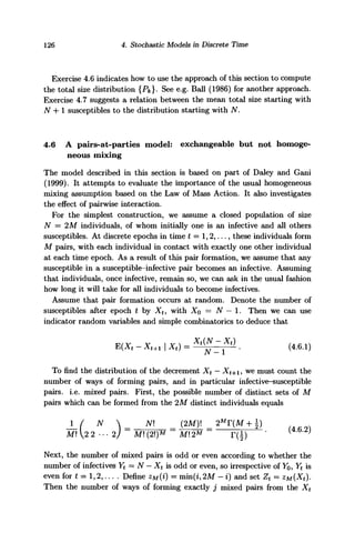
139. 4.6. A pairs-at-parties model 127
susceptibles and Yt infectives is zero if Zt + j is odd, and
(Zt (2M — Zt ( the number of ways of forming
V 3 ) 3 ) (z
t~ j) and M - {Zt + j) non-mixed pairs/
Ztl(2M-Zt) (Zt-j)
j (Zt - j) (2M - Z t - j) (Zt - j})
(2M-Zt-j)
- (4.6.3)
otherwise. It now follows that the one-step transition matrix for the Markov
chain {Xt : t = 1,2,...} has elements Pi^-j = rj(i,M) where, with Zt =
above,
rj(i, M) = Pr{Xt+1 =Xt-jXt = z, M}
(2M-Zt-j)fZA (2M - Zt j(Zt-j)
j ) 3 )(±[Zt-j))2^-
(2M)!
M!2M
2J'Zt!(2M-Zt)!M! =
2J
'(,- i(zt-j)V^(zt+j))
j ([Zt - j)) (M - Zt + j])! (2M)! (2
^)
C7 = Z f , Z t - 2 , . . . , l o r 0 ) ,
0 otherwise.
(4.6.4)
We can now use this Markov chain to find numerically the distribution of
the time T until all 2M individuals are infective.
The assumption that transmission of infection occurs in every infective-
susceptible pair is unrealistic. If infection occurs with probability /?' say,
then by using indicator variables we should have in place of (4.6.1) the
relation
Y P'Xt(N - Xt)
X) =
(4.6.5)
The transition probabilities V^i-j sav
> a
re
now binomial mixtures of the
terms r^(z, M), because from the random number Kt of mixed pairs formed
by the Xt susceptibles and N — Xt infectives, the number of new infectives
is a binomially distributed r.v. Bn^i^,/?'). We have
min(i,N-i) .
( (4.6.6)
=3

140. 128 4. Stochastic Models in Discrete Time
1
1 —
0.8-
0.6-
0.4-
0.2-
o
1
1
1
<
1
1
1
1:,1
0 10
/
/
/
/
/
1
1
1
1
i
20
/ '
/
1
30
1
40 12
(a) (b)
Figure 4.3. Duration time distributions for the pairs-at-parties model with
0' = 1 ( ), /?' = 0.5 ( ), and ff = 0.3 ( ), for N = 20.
(a) Actual time Pr{Xt = 0}, (b) rescaled time Pr{Xt/(3f = 0}.
Figure 4.3 plots the distrubution of the duration time of an epidemic in this
model for three values of /?', with values rescaled in part (b) of the figure
indicating convergence as f¥ | 0 to a limit in which the effect of exactly M
pairs being formed in each time unit largely disappears. These distributions
can also be illustrated by plotting the mean numbers of new infectives in
a time unit (see Figure 4.4). Rescaling again emphasizes similarities and
suggests convergence (see Exercise 4.8).
We now attempt to understand better the effect of the pair-formation
aspect of the model relative to 'classical' homogeneously mixing models,
subject of course to appropriate choice of such a classical-style model. For a
start, we observe that in the pairs-at-parties model every individual in the
closed population is either susceptible or infective, and that once infected, an
individual remains so forever. In this respect the model resembles the simple
stochastic epidemic X(t) of Section 3.1 starting from N — l susceptibles and
1 infective, with transmission rate /? which we must determine appropriately.
We deduce from Section 3.1 that
d_
(4.6.7)
we can immediately see the similarity of functional form with the right-hand
side of (4.6.5). This derivative best approximates the discrete-time mean
decrement at (4.6.5) (which includes the case /?' = 1 in (4.6.1)) by setting
P = (3'/(N — 1). The deterministic analogue of this stochastic model gives
the logistic growth curve as in Section 2.1.

141. 4.6. A pairs-at-parties model 129
However, since the pairs-at-parties model is a discrete-time model, with
exactly M = N pairs formed in each unit of time, we should use a discrete
time analogue of this simple epidemic model. We consider two possibilities.
For the first we start with the discrete time approximating process
defined by X$ = N — 1 and the one step transition probabilities
if j = i,
otherwise.
(4.6.8)
We recognize that the term Pi,i-i equals the product of the probabilities
that a randomly chosen pair is a mixed pair and that there is infection
transmission. Since M pairs are formed in each time unit of the pairs-at-
parties process {Xt} it is appropriate that it be compared with the process
{Xt} =
5 -
4 -
o
2 —
1 -
0 -
/ ,
/ /
/ /
it
/
1
0 2
/~v
i
4
1
1
6
1
8
1
10
_
"I12
(a)
2 -
1 . 5 -
0 . 5 -
u
(
/
ilif
ij
)
/
/
i
5
A
10
I
15
1
20
1
25
(b)
Figure 4.4. Mean numbers of new infectives in pairs-at-parties model
( ), approximating discrete simple epidemic model ( ), and
approximating Reed-Frost-style simple epidemic ( ), for iV = 20
and (a) ff = 1, (b) ff = 0.5.
Figure 4.4 compares the two processes {Xt} and {Xt} for N = 20 and
the two cases /?' = 1 and /? = 0.5, plotting for each time unit the mean
decrements E(Xt — Xt-), i.e. the mean numbers of new infectives. The
figure also shows the corresponding data for the other discrete-time pro-
cess {Xt} that is a simple epidemic analogue of the Reed-Frost model of
Sections 4.1-2. Conditional on Xti Xt+i is a binomially distributed r.v.

142. 130 4. Stochastic Models in Discrete Time
, qN
~Xt
), where q denotes the probability that a given susceptible is
not infected by a given infective in the time interval (t, t + 1). This process
Xt has mean decrement
E(Xt - Xt+1 | Xt) = Xt[ - = Xtp{ + q
^Xt(N-Xt)p. (4.6.9)
By choosing p = (3'/(N — 1) we approximate the decrement (4.6.5), exactly
for X^ = N — 1 = XQ] otherwise (4.6.9) is a lower bound. Thus, we could
expect this simple epidemic analogue of a Reed-Frost epidemic to evolve
more slowly than the pairs-at-parties model.
Figure 4.5 provides another comparison of the processes {Xt}, {Xt} and
{Xt}, by plotting the increments Pr{Xt = 0} - Pr{Xt_i = 0} of the d.f.
shown in Figure 4.3, in the two cases /?' = 1 and 0.5 as for Figure 4.4. Figure
4.4 indicates that the spread of infection in the pairs-at-parties model is
more rapid than the Reed-Frost simple epidemic analogue, as noted below
(4.6.9). Compared with the simple epidemic analogue, its initial spread is
slower; in the middle and later stages, however, its spread is faster so that
the population becomes totally infected more rapidly (this latter point is
underlined in Figure 4.5).
0.6-1
0 . 4 -
0 . 2 -
0.15-
0.1-
0.05-
o -
(
1
J1
) 5
/
I1
;
//
I
10
1
15
1
20
^.
1
25
(a) (b)
Figure 4.5. Increments Vi{Xt = 0} — ¥x{Xt~ = 0} in the duration time
distribution of pairs-at-parties model ( ), approximating discrete simple
epidemic model ( ), and approximating Reed-Frost-style simple epi-
demic ( ), for N = 20 and (a) ff = 1, (b) ff = 0.5.
Decreasing (3f
has the effect of increasing the uncertainty of transmission
of infection. All three Figures 4.3-5 indicate that as /?' decreases, the pairs-
at-parties model resembles a classical model more closely.

143. 4.7. Exercises and Complements to Chapter 4 131
By way of summary, these properties indicate that, compared with stan-
dard homogeneous mixing models, an epidemic spread via the 'regulariza-
tion' of pair-formation for all individuals in each discrete time unit, leads
to a more predictable and ultimately faster spread of infection. However,
the effect of pair-format ion in each time unit is not great.
4.7 Exercises and Complements to Chapter 4
4.1 (a) Use a sketch graph to check that when (4.4.9) holds, the root £ of equation
(4.4.10) lies between N and £0 = Nct(l - p)/(l - pa).
(b) Expand the term qN
~* when (N - £0)| ln(l - p) is small (i.e. (N - £0)p
is small) and deduce that
Compare with the numerical values in Table 4.4.
4.2 Show that for a stationary process {Xt} satisfying (4.4.11),
[1 - (pet)2
] var X = a(l - a)(N - pEY) + a2
pqEY,
where Y — N — X. What is the asymptotic behaviour of 1 — w for large Nl
Investigate conditions for a 'quasi-stable' Y that is O(l).
4.3 Compare the stationary mean EX at (4.4.13) with the least root f of (4.4.10)
given in Table 4.4.
4.4 Investigate whether martingale and/or transform methods may assist in
studying the process {Xt} of Section 4.4, in particular first passage time
variables and the value of £ (or other quantity) as an approximation.
4.5 Show that the total size distribution {Pk} of an epidemic starting from /
infectives and otherwise as in Section 4.5 can be computed from

144. 132 4. Stochastic Models in Discrete Time
4.6 (a) Show that the total size distribution {Pk} of the stochastic carrier epi-
demic model of Section 3.6 can be computed from Pk = Pn-k,o where, start-
ing from Pnb — 1, the quantities PtJ = Pr{for some t there are i susceptibles
and j carriers} are defined recursively by
Pib =Pt+iP<+i,6 (i = n - l , . . . , 0 ) ,
Pnj =qnPn,j + l (j = 6 - 1, . . . , 0),
Ptj = Pt+iPt+i,j + QiPt,j+i (i = n - 1,. •.,1; j = b - 1,..., 1),
in which pt = i/(i + p) = 1 — qt.
(b) Justify the alternative computational scheme based on Pk = P^-k w n e r e
p^ = Sm and for j — 6,..., 1 and i = n,..., 0,
ti /
[Reinarlc: Either of these computational schemes is numerically more stable
than the explicit formula at (3.6.12).]
4.7 In the Markovian model for a general stochastic epidemic process {(X,Y)t :
0 < t < oo} discussed in Section 3.3, starting from (X,Y)0 = (TV, 1), let
Ht denote the increasing a-fields determined by the sample paths {(X, Y)u :
0 < u < t}. Regard a similar model (X,Y)t with (X,Y)o = (N + 1,1) as
starting with the same (N, 1) individuals as determine Ht augmented by a
distinguished individual that is initially susceptible and that has no impact
on the sample paths (X, Y)t for precisely as long as it remains susceptible.
Show that
PN+i(t) = Pr{distinguished individual is susceptible at t}
= E[exp(-/?/o
t
y(«)dU )|Ht ].
Prom this it is plausible that
7
TV + 1
compare with the argument in Ball (1986). Cf. also (2.3.7) and Exercise 5.6.
4.8 Investigate appropriately rescaled limits of the pairs-at-parties model and
of the two simple epidemic analogues of Section 4.6, for (a) TV —> oo, and
(b) ff - 0.

145. Rumours: Modelling Spread and its Cessation
This chapter is devoted to further models of spread in a population, most
of them appealing to the Law of Mass Action. Our aim is to exemplify the
modelling principles found useful in other problems involving the spread of
an attribute through a population. It is important to note that except for
models in which the only 'mechanism' is that of spreading, as for example in
the case of a simple epidemic, the range of behaviour exhibited by processes
with a removal mechanism is quite varied.
The two key features of previous models involve the spread of a disease
and the removal of infectious individuals. We have given some emphasis in
Chapters 2, 3 and 4 to the spread of disease by other than homogeneous
mechanisms. In this chapter we look also at a variety of removal mecha-
nisms, such as may apply to the spread of a rumour (an 'infection of the
mind'). We show that different removal mechanisms can lead to somewhat
different conclusions from those of earlier chapters, where threshold phe-
nomena were of particular interest.
5.1 Rumour models
The earliest references in the probability literature to a rumour model
appear in the work of Rapoport and co-workers from 1948 onwards (see
Bartholomew (1967) for references), in Feller (1957, Exercises 11.10.21-22)
though not in his first (1950) edition, and in Kendall (1957). Here we take
as our basic model that described in Daley and Kendall (1965) (called [DK]
below), where the original motivation for its formulation was the possible
similarity in the spread of physiological and psychological infections (cf.
Daley and Kendall, 1964). The analysis that ensued highlighted a major
difference in modelling the way that spreading ceases for the two types of
'infection'.
133

146. 134 5. Rumours: Modelling Spread and its Cessation
As in the simpler models of Chapters 2 and 3, we consider a closed ho-
mogeneously mixing population of N -f 1 individuals. At any time they can
be classified as belonging to one of three mutually exclusive and exhaustive
categories consisting at time t > 0 of
(a) X(t) individuals who are ignorant of the rumour;
(b) Y(t) individuals who are actively spreading the rumour; and
(c) Z(t) individuals who know the rumour but have ceased spreading it.
Initially, X(0) = N, Y(0) = 1 and Z(0) = 0, while for all t, X(t) + Y(t) +
Z(t) = N 4- 1. We refer to these three types of individuals as ignorants,
spreaders and stiflers respectively; they are the equivalents of susceptibles,
infectives and removals of the general epidemic model of Chapter 3, but we
model their behaviour somewhat differently.
The rumour is propagated through the population by contact between
ignorants and spreaders, following the law of mass action just as in Chapter
3. Specifically, assume that any spreader involved in any pairwise meeting
attempts to 'infect' the other individual involved in the meeting; this 'other
individual' is either an ignorant, a spreader or a stifler. In the first case,
the ignorant becomes a spreader; in the other two cases, either or both of
those involved in the meeting learn that the rumour is 'known' and so decide
not to tell the rumour any more, thereby joining the stiflers as a result of
this 'stifling experience'. When the pairwise meeting rate is /?, ignorant-
spreader, spreader-spreader and stifler-spreader meetings occur at time t at
relative rates 0X(t)Y(t), f3Y{t)[Y{t) - 1], and (3Y(t)Z(t) respectively. It
is convenient to write such changes as may occur in a (small) time interval
(t, t + h) in the form
Ah(X, Y)(t) = (X, Y)(t + h) - (X, Y)(t), (5.1.1)
so for example an ignorant-spreader meeting yields Ah(X, Y)(t) = (—1,1).
We use the meeting rates to set the transition rates for changes in the state
of the population, and so deduce the relations, with the approximations
neglecting terms that are o(h),
Pr{Afc(X, Y)(t) = (-1,1) | (X, Y)(t) = (x, y)} = 0xyh,
Pv{Ah(X,Y)(t) = (0,-2) | (X,Y)(t) = (x,y)} = j3y{y - l)h,
Pr{Ah(X, Y)(t) = (0, -1) | (X, Y)(t) = (x,y)} = 0yzh, (5.1.2)
Pr{Ah(X, Y)(t) = (0,0) | (X, Y){t) = (x, y)} = 1 - 0y(N - [y - l])h,
while all other transitions have probability o(h). It is clear here that (3
plays the role of a time constant, so by suitable choice of time unit we may
assume that (3 — 1.

147. 5.1. Rumour models 135
We shall be interested in the proportion / of the ignorant population
X(0) = N which eventually learns the rumour, so that
Km X(t) = N-Nf, limr(t) = 0, lim Z(t) = 1 + Nf. (5.1.3)
t—+oo t-+oo t—*oo
We can study the properties of / both in a deterministic version of the
model described by equations (5.1.2) (cf. Chapter 2 and Section 5.2 below),
and an embedded jump chain argument (cf. Sections 3.4.2-3 and 5.3). It is
also convenient to use the present context to describe an argument due to
D.G. Kendall leading to a quicker computation of asymptotic properties of
the model for larger population sizes (see Section 5.4).
We now describe two simple variants of the basic [DK] model. For the
first, which we call the A:-fold stifling model, assume that a spreader does
not decide to stop propagating the rumour until being involved in A: stifling
experiences as described earlier. Then by identifying the Y(t) spreaders as
belonging to one of the k mutually exclusive categories of spreaders who
have had j stifling experiences (j = 0,..., k — 1), we can still give a Marko-
vian description of the process, using the larger, (k + l)-dimensional vector
(X, Yi,..., Yk)(t) where (Yx + • • •+ Yfc)(*) = Y(t) = N+ 1-X(t) - Z(t) as
earlier. See Exercise 5.3 for a deterministic version of this model.
For the second variant, which we call the (a,p)-probability variant, ob-
serve that the [DK] model is certainly simplistic in supposing that (a) every
pairwise meeting involving a spreader results in the spreader attempting
to spread the rumour, and (b) a spreader becomes a stifler as a result
of exactly one stifling experience. Suppose instead that a spreader in-
volved in a pairwise meeting attempts to spread the rumour with prob-
ability p, and that when such an attempt is made any spreader so in-
volved decides with probability a to become a stifler, independently for
each spreader and each meeting. The basic model has p = a = 1; we now
suppose that 0 < p < 1 and 0 < a < 1. Then when (X,Y)(t) = (x,y),
there occurs in (t, t + h) either an (X, Y) meeting resulting in A^(X, Y) =
(—1,1) with probability pxyh (neglecting o(h) terms), or a (Y,Y) meet-
ing resulting in A/^X, Y) = (0, -1) or (0, -2) with respective probabilities
p(2 - p)a(l - a)y(y - l)h and p(2 - p)a2
y(y - l)/i, or a (Y", Z) meeting
resulting in Ah(X, Y) = (0, -1) with probability payzh, or no change with
probability 1 - p[(l + a)x + (1 - p)a(2 - a)(y - l)]yh.
Another model which has gained some currency, if only because of its
simplicity and appearance in an undergraduate text, is due to Maki and
Thompson (1973). As before, the population is classified and counted as
(X, Y, Z); a continuous time Markov process version of the model is then

148. 136 5. Rumours: Modelling Spread and its Cessation
as follows (Watson, 1988). The rumour is spread by directed contact of the
Y(t) spreaders at time t with others in the population. The outcome of
contact of a specified spreader with (a) an ignorant is that the ignorant be-
comes a spreader, and (b) another spreader or a stifler, is that the initiating
spreader becomes a stifler. No other micro-level transitions occur. Then
the model has just two elementary transitions, with Ah(X,Y) = (—1,1)
or (0, -1) at infinitesimal rates XYh + o(h) and Y(Y - 1 + Z)h + o(h)
respectively, i.e. omitting terms o(/i),
Pr{A*(X, Y)(t) = (-1,1) | (X, Y)(t) = (s, y)} = xyh,
Pr{A^(X, Y)(t) = (0, -1) | (X, Y)(t) = (*, y)} = y(y + s - l)/i, (5.1.4)
Pr{A*(X, y)(*) - (0,0) | (X, y)(«) = (*, y)} = 1 - Nyh.
Notice that because there is now directed contact of the initiating spreader,
the term y(y — l) of equations (5.1.2) is replaced by y(y — l) in (5.1.4). The
model is otherwise like the [DK] model in assuming that it is only through
interaction between the initiating spreader and others of the population that
a spreader becomes a stifler. The resulting deterministic analysis is similar
(see the next section and Exercise 5.4), but not so the stochastic analysis
(see Section 5.3 and Exercise 5.7).
Both the simple epidemic model and the general epidemic model discussed
in Chapter 3 have been suggested as models to describe the spread of a ru-
mour (e.g. Goffman (1965), Goffman and Newill (1964, 1967), Bartholomew
(1973, Chapters 9 and 10)). Recall that the general epidemic model has
two basic transitions possible in a small interval of time of length /i, namely
A/j(X, y) = (—1,1) or (0, —1) at rates (3xy and 72/ respectively. Clearly the
first transition can result from an (X, Y) contact, but the second requires
no interaction between individuals in the population at all. It is enough for
the cessation of rumour-spreading to occur purely as a result of a spreader's
'forgetting', irrevocably, to tell the rumour to those of the population with
whom (s)he comes into contact. Now forgetfulness, or disinclination ever
to tell the rumour, are certainly features we may wish to model as factors
contributing to the decline in the spread of the rumour. But it seems an
unrealistic description of human behaviour to make it the sole mechanism
causing the cessation of a rumour's spreading, in the same way as total
reliance on the stifling mechanism may be unrealistic. Just as diseases may
vary in their potency, so rumours may vary in the urgency with which in-
dividuals communicate them. On balance we may wish to use both stifling
and forgetfulness mechanisms (for surely, some items of news are eminently
forgettable!); one possible way of doing so is indicated in Exercise 5.5. It

149. 5.1. Rumour models 137
would then be reasonable to expect the relative rates of pariwise contact
(for both spreading and stifling) and of individual forgetfulness to affect the
extent of the spread of the rumour.
Threshold phenomena such as occur in branching processes or the spread
of epidemics (see e.g. Chapters 2 and 3) depend on a balance between
spreading on the one hand and cessation of spread on the other. If, as in
the basic [DK] models, the cessation depends on interaction of the spreaders
with themselves or stiflers in the population, then the effect of the cessa-
tion mechanism is negligible relative to that of the spreading mechanism
when the numbers of spreaders and stiflers are small. On the other hand,
when cessation of contagious spread occurs as a result of the evolution of
a spreader independently of the rest of the population, with spreading de-
pendent on the state of the population, then it is the state of the rest of the
population, relative to the dynamics of spread and its cessation amongst the
spreaders themselves, that determines the fate of the spread. In this case,
conditions for threshold criteria exist, whether for the spread of a disease
or a rumour, as in the general epidemic model.
We now describe a distinctly different family of models for the spread
of news or a rumour in a population. For convenience we assume that
the population is of constant size N + 1, its members being classified as
ignorants, spreaders and former spreaders (e.g. stiflers or removed cases),
much as before; initially there are N ignorants and 1 spreader. Let each
individual becoming a spreader, including the initial spreader, be identi-
fied by a distinct integer-valued index r. Spreader r spreads the rumour
to Kr individuals chosen at random (without replacement, for definiteness)
from the rest of the population; {Kr : r — 1,2,...} is a family of indepen-
dent identically distributed integer-valued random variables with distribu-
tion {fk = Pv{Kr = k}, k = 0,1,...} and mean m = EKr. Those of the
Kr individuals who are ignorants become spreaders, while the others are
not affected by the contact. After making these Kr contacts, spreader r
plays no further part in spreading the rumour. A convenient identification
of the indices is that matching the order in which the r.v.s {Kr} are taken
into the analysis. Then, writing (Xr,Yr) for the numbers of ignorants and
spreaders just before the Kr contacts occur, we have for Yr > 1,
Xr + 1 =Xr- Jr(Kr), Yr+1 =Yr-l + Jr(Kr), (5.1.5)
where Jr(Kr) denotes the number of contacts with ignorants amongst the

150. 138 5. Rumours: Modelling Spread and its Cessation
Kr contacts of spreader r. These assumptions give
K) -11 *=o - 1 AG)(*:;)/CO • (5L6)
K—J
for r such that Yr > 1. Recognizing the hypergeometric distribution prob-
abilities as the coefficients of /&, we have E(Jr(Xr) | Xr = i,Yr > 1) =
Sfc fkk{i/N) = mXr/N. The relations (5.1.5) are similar to those at equa-
tion (4.5.2) where we considered the analysis of a variant of the general
epidemic model by means of an embedded random walk. The same ap-
proach is applicable here.
Such a model is most aptly described as a branching process on a fi-
nite population. It can certainly be used to describe the so-called chain
letter process. It also includes the general epidemic model when {/&} is
the geometric distribution {pNk
~1
/(N + p)k
: k = 0,1,...}) as far as the
ultimate extent of the spread of the news or rumour is concerned. There
exist both deterministic and stochastic threshold theorems for which a ma-
jor outbreak can occur only if m > 1. Chapter 10.3 of Bartholomew (1973)
includes discussion that refers to related work of Rapoport and co-workers.
5.2 Deterministic analysis of rumour models
Except for the branching process model described at the end of the last
section, the models we have sketched for the spread of news or a rumour
can be formulated as Markov processes in continuous time. Their analysis
by explicit algebra does not proceed easily; in particular their transition
probabilities are not readily accessible for the range of parameter values of
interest, most notably the initial number of ignorants N. We resort in the
first instance to deterministic versions of the models.
For the deterministic version of (5.1.1) we consider the continuous func-
tions x(t), y(t) and z(t), differentiate in t, that have the same initial val-
ues x(0) = X(0) = N, y(0) = Y(0) = 1, z(0) = Z(0) = 0 and satisfy
x(t) 4- y{t) 4- z(t) — N 4-1 for a closed population. The rates of change of
x and y are assumed to coincide with the rates of change of the conditional
mean functions such as lim^o E(X(t + h) | (X, Y)(t) = (i, j)) at the lattice
points (£, j), 'smoothly' interpolated between. These limits are assumed to
be given as below:
x = ^ (change in x) x (rate of change) = (—l)xy, (5.2.1a)
simple transitions

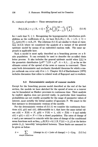
151. 5.2. Deterministic analysis of rumour models 139
and similarly,
y = (+i)xy+(-2)Iy (v -l)+(-l)i/« = 2/(x-2/+l-z) = y(2x-N). (5.2.1b)
These two equations yield
^ = - 2 + ^ , (5.2.2)
dx x
whose solution consistent with the initial conditions is
2x(t) + y{t) + NIn - ^ = A(a(t), j/(t)) = 2JV + 1 (all t > 0). (5.2.3)
x{t)
It follows from (5.2.3) that the limit lim^oo x(t)/N = ON say, analogous to
the proportion / at (5.1.3) of ignorants who never hear the rumour, satisfies
-1 = 2AT(1 - 0N) + NlnONi (5.2.4)
and that liniAr-*oo ON = 0 satisfies
2(1-0) +In 0 = 0. (5.2.5)
This is the same as the equation for the deterministic model of a general
epidemic considered in Chapter 2.3, having relative removal rate ^N (cf.
equations (2.3.6) and (2.3.7)). Unlike the epidemic model, the rumour model
no longer has a family of processes with a parameter determining threshold
behaviour. Instead, the analogy is with a single process; it is not difficult
to check that the dependence on N of the root ON of (5.2.4) is O(N~l
) (see
Exercise 5.1).
In a similar fashion, the general (a,p)-probability variant of the basic
[DK] model leads to the pair of differential equations
x = (~l)pxy,
y = (+l)pxy + (-l)[p(2 - p)2a(l - a)y(y - 1) +payz]
+ (-2)p{2-p)a2
y{y-l)
In this case, the analogue of equation (5.2.2) is
^ = _{1 + a)+a(N-l+P)+a(l-P)y
dx x x

152. 140 5. Rumours: Modelling Spread and its Cessation
1 -
0 . 8 -
0.6-
0.4-
0.2-
0.001 0.01
0.0001
0.05 0.10 0.15 0.203 0.25
Figure 5.1. Contours of 0(a,p), the proportion of a large population not
hearing a rumour with uncertain spreading (p < 1) and stifling (a < 1). The
values at the top of each curve are of 0(a,p), the smaller positive root in 0
of equation (5.2.8) (see Exercise 5.2 for 0max).
This is still a first order linear differential equation, with the general solution
(1 + a)x N
V
~~ l - a ( l - p ) 1-p N
^pX
for some constant XN,Q,P of integration which is determined by the initial
conditions, yielding
(l4-cy)r N
11 T ulX IV
The proportion 0N of ignorants who never hear the rumour behaves much
as the root of equation (5.2.4), but with limit 0 = 6(a,p) — linijv^oo ON
now satisfying
(2 - - p)0 = 1 - a(l - p). (5.2.8)
The contour curves in Figure 5.1 depict the non-unit root 0(a,p) as a func-
tion of a and p; always, 0 < 0(a,p) < 0max, where 0max « 0.284668 is the
smaller positive root of 0(1 - 2 In 0) = 1 arising from the limit a -> 1 and
p —> 0 (see also Exercise 5.2).
The deterministic analysis of Maki and Thompson's model is sketched in
Exercise 5.4.

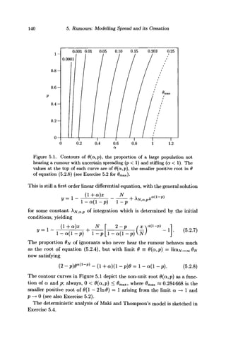
153. 5.3. Embedded random walks for rumour models 141
5.3 Embedded random walks for rumour models
We now return to [DKj's stochastic model described by the Markov chain
with infinitesimal transition rates as at (5.1.2). The main vehicle for study-
ing the final state of this process (e.g. [DK] and Pittel (1990)) has been the
Markov chain embedded at the jump points occurring at times t,... ,£n,
... ,1M (cf. Section 3.4.2 above), where M is the total number of jumps.
We note that because the state space is finite and the process is 'strictly
evolutionary' in the sense of having well-ordered sample paths, M must be
finite.
Denote the states immediately after these jump epochs by {(X, Y)n : n =
0,1,...}, with (X, Y)o = (iV, 1), so that when for some particular n we have
{
(—1, +1) with probability i/fij,
(0, -1) with probability (N+l-i- j)/fih
(0, -2) with probability (j - l)//y ,
(5.3.1)
where fij = N — ^(j — 1). Note that the first case is excluded if i — 0,
when the probability equals zero, or j = 0, while the last case is excluded if
j < 1. This embedded jump process is a random walk on that part of the
two-dimensional integer lattice for which 0<i<N,0<j < 7V+1 — i, and
the states {(z, 0) : i = 0,..., N - 1} are absorbing. Prom equations (5.3.1)
we can derive equations for the probabilities P^ on the path of a rumour,
defined by
Pit = Pr{(X, Y)(t) = (ij) for some t}
= Pr{(X, Y)n = (i,j) for some n}. (
' ' j
The Markov process {(X,F)(£)} is strictly evolutionary in the sense that,
once a state (z, j) is visited and left, it is never visited again. Hence the prob-
abilities P^ satisfy a set of equations, derived by a forward decomposition
argument, of the general form
jump is A | present state is (ij) - A}, (5.3.3)
where A denotes one of the three jumps (-1,1), (0,-1) and (0,-2) at
equation (5.3.1). Specifically, starting from PNi = PN-I,2 = 1, we have for

154. 142 5. Rumours: Modelling Spread and its Cessation
N-i + D, (5.3.4a)
(J = N- *), (5.3.4b)
J V $ ( j + l ) P f J + a
(2 < j < N - 1 - i), (5.3.4c)
From these relations, in the same way as the distribution of the size of
the general epidemic process was derived in Section 3.4.3, we can find the
distribution
{Pio} = {Pr{rumour ends with i ignorants} : i = 0,1,..., N - l}. (5.3.5)
Figure 5.2(a) illustrates the complementary distribution {PN^iy0} of the
number of ignorants hearing the rumour in this model, for two initial sizes
N = 50 and 100. The scales have been changed as indicated in the figure
for N = 100, to facilitate comparison of the two distributions.
In [DK] it was concluded that the proportion £/v = X(oo)/N of ignorants
left when the rumour stops spreading has
E£N « 0.203188 + 0.273 843/JV = 0 + 0.273 843/iV,
JVvax^« 0.310681 +1.232 700/JV.
Observe that the correction term added to 9 — 0.203188, the solution of
equation (5.2.5), shows that ON, the solution of (5.2.4) (see Exercise 5.1),
is such that ON ^ E£/v, nor is there any good reason that equality should
hold. In Section 5.4 we note that
= 0.310681 ««»„«„. ,5.3.7,
For the [DK] model the general form of equation (5.3.4) involves three
terms on the right-hand side. For the Maki-Thompson model, however,
while the same deterministic equation (5.2.2) applies, the analogous equa-
tion has only two terms, corresponding to the simpler possible transitions

155. 5.3. Embedded random walks for rumour models 143
0.15
100
0.05
0.15
0.05
10 20 30 40 50 0 10 20 30 40
(a) [DK] model (b) Maki-Thompson model
Figure 5.2. Frequency polygons of the distribution of the numbers of
ignorants ultimately hearing a rumour in two rumour models, for N = 50
( , scales as shown) and N = 100 ( , double the abscissa scale, halve
the ordinate scale, as indicated at top right-hand corners).
as at (5.1.4). Specifically, starting from
now have for i = 0,..., N — 1,
= P/v-1,2 = 1 as before, we
N
1),
j = 0,l).
(5.3.8a)
(5.3.8b)
(5.3.8c)
In principle, generating function methods could now be used to study these
equations and develop a routine for evaluating Pi0. But it is unquestionably
more practical to proceed directly to their numerical evaluation (see Table
5.1 for some values of moments), and to contrast their stochastic behaviour
for larger N using the diffusion arguments presented in Section 5.4 (cf.
Exercise 5.7). By fitting quadratics in 1/N to the last two columns of Table
5.1 for N = 191, 383 and 767, we obtain in place of (5.3.6)
N var 6v
0.203188 + 0.117 20/iV + 0.6606/iV2
0.272 735 + 0.529 86/AT + 5.5823/iV2 (5.3.9)
These results differ from the relations at (5.3.6) for the [DK] model except
for the commonality of 0 = 0.203188 in E£N. The values for N in the table
are used to facilitate direct comparison with [DKj's Table 1. Note that the
moments given are of X(oo) conditioned to be less than N — y/N: condi-
tioning is necessary because otherwise the term PN-i,o = I/AT2
contributes

156. 144 5. Rumours: Modelling Spread and its Cessation
Table 5.1. Maki-Thompson model: mean and variance
of ultimate numbers of ignorants remaining
N
95
191
383
767
EX(oo)
19.4274
38.9295
77.9398
155.963
varX(oo)
26.5051
52.6515
105.002
209.725
0.204499
0.203819
0.203498
0.203342
N var £N
0.279002
0.275662
0.274155
0.273435
significantly to var£/v- The result would then belie the description of the
distribution as approximately normal, and would be reminiscent of the ma-
jor/minor humps of the final size distribution of the general epidemic (cf.
Figure 3.2). Pittel (1990) illustrates ways around the complications that
result from this fact when attempting to use a moment method for proving
asymptotics of the final size distribution. Watson (1988) remarks that the
fact that the asymptotic value of NVSX£N for the Maki-Thompson model
is smaller than for the [DK] model 'accords with the change to smaller more
frequent jumps in the removal process'.
Figure 5.2(b) complements part (a) by presenting the distribution for the
Maki-Thompson model. The probability of very few ignorants ever hearing
the rumour, which is approximately ^N~l
for the [DK] model and N~2
for
the Maki-Thompson model, shows as a small peak in (a) and not at all in
(b), at the scale of the diagram and for the values of N used.
Both the general epidemic and Maki-Thompson models have embedded
random walks that are of a simpler structure than that in the [DK] model.
Specifically, because the process is strictly evolutionary and the jumps are
to 'adjacent' states, much as in a birth-and-death process, the 'time' argu-
ment n of the embedded jump process can be used to reduce the dimension
of the state space, from a two-dimensional to a one-dimensional lattice. To
study such processes we replace the embedded jump process {{X,Y)n} by
{(X',Y')n] which is defined as starting from the same initial state and as
having one-step transitions to (-1,1) and (0,-1) with the same probabili-
ties as for {{X,Y)n}. But now {{XY')n} is no longer confined to a first
passage into the states (0,j) (j = 0,..., N); rather,
(X Y')n - (X Y
Clearly, (X, Y)n = (X Y')n for n = 0,..., Af.
Now, after n jumps starting from (X',Y')0 = (N, 1), it must be the case,
since these n jumps have increments that are either (-1,1) or (0, -1), that

157. 5.4. A diffusion approximation 145
n = N - X'n + (1 4- N - X'n - Y£), or 2X'n + Y^ + n = 27V + 1. Prom this
relation we deduce that M = inf{n :n = 2N + 1 — 2X'n).
Also, conditional on the <j-field Tn = O~(XQ, ..., X'n), the expected decre-
ment in {X'n} equals X'JN, or equivalent^, E(Xn+1 | ^n ) = Xf
n{ -N~l
).
This means that the functional Vn = [N/(JV - l)]n
X^ satisfies
N
x'n) = [ ( T )
L V 7 V i y
J (5.3.II)
implying that {Vn} is a martingale with respect to the cr-fields {.Fn} o n
which M is a stopping time.
Similarly, E([X;+ 1 - X^]2
| ^ n ) = X'JN so that
and
and therefore {[AT/(AT - 2)]n
(X;2
- X^)} is also a martingale.
Sudbury (1985) uses this pair of martingales in conjunction with the
stopping time M to prove that as N —> oo, £# ~~> ^ m
probability. This
is a weaker statement than the convergence in distribution of /N(^N - 0).
Exercise 5.6 sketches a pair of martingales for the analogous embedded jump
process {(X;
, Y')n} defined on a general epidemic.
5.4 A diffusion approximation
Daley and Kendall (1965) outlined an heuristic method for evaluating
var X(oo), the variance of the number of ignorants remaining when spread-
ing stops. The major step in the procedure is to find the variation in A,
the stochastic analogue of the deterministic 'constant of integration' A in
(5.2.3). We describe the mechanics of the procedure; mathematical details
of the martingale and limit arguments involved can be found in Barbour
(1972, 1974) and e.g. Watson (1988). Martingale arguments have also been
noted by Pittel (1990) and Lefevre and Picard (1994).

158. 146 5. Rumours: Modelling Spread and its Cessation
The essence of Kendall's Principle of Diffusion of Arbitrary Constants,
as it applies to pure jump Markov population processes such as epidemics
or predator-prey models, embodies two features, one reflecting the mean
behaviour of the process and the other the variability about that mean
behaviour. The mean behaviour is represented by the so-called determin-
istic path or deterministic version of the model; ideally, this is represented
by an 'invariant of the motion', to borrow a phrase from classical applied
mathematics. Its probabilistic analogue is a martingale. The variability can
be regarded as a diffusion on adjacent paths, each path characterized by a
different starting point. The local probabilistic analogue is the quadratic
variation of the martingale. The total variation is then the result of accu-
mulating this local variability as the process evolves along its deterministic
path.
In the rest of this section we illustrate this approach as it applies to the
[DK] rumour model and the general epidemic. Three more applications are
stated as exercises.
By analogy with (5.2.3), but recalling that the rumour process (X,Y)(t)
is lattice-valued, we start by writing
l (5-4.1)
{X(t),Y(t)) = 2X(t) + Y(t) ^
where A() is clearly a random variable. Recall from (5.2.3) that X(t) =
(x(t),y(t)) = 2x(t)+y(t)-Nln[x(t)/N] = 27V+1 (alH > 0) for (x(t),y(t))
denoting the deterministic path. We use this relation later in the form
y(t) -1 = 2[N- x{t)} + JV In ^ . (5.4.2)
Now the process A(t) is a martingale with respect to the cr-fields {^i-} =
{a({(X, Y)(s) : s < £})}, as is verified by evaluating
E(dA(t) | Tt-)
= [(-! + j^))x
Wy
W +
i-iWW) + (-2)iy(t)[r(t) - i]l dt
= Y(t) (N -X(t)- Z(t) - Y(t) + 1) dt = 0. (5.4.3)
To find its quadratic variation we find E([dA(£)]2
| Ft-), namely
-Y(t)Z(t) + 2Y(t)[Y(t)-l]dt
= Y(t)^N-2N+-~+Y(t)~l]dt. (5.4.4)

159. 5.4. A diffusion approximation 147
In order to compute the total quadratic variation over the evolution of
the spread of the rumour, we replace the stochastic process (X, Y)(t) on the
right-hand side by its deterministic version (x(t),y(t)) given by equation
(5.4.2) with N > x(t) > NO and x(t) = -x(t)y(t). These substitutions give
fN
var A(oo) « /
Jx=N0
N2
x
- I - TV + — + 2(N - x) + ATln ± I dx
Ar f1
l
= N /
7^
dtx
= Ar( i-g)(i-2g + ag»)> ( 5 4 5 )
using (5.2.5) at the last step. Since d/dxx=Ne = (1 — 20)/0, we arrive
finally at
varA(oc)« ^ L _ i, (5.4.6)
which is the source of the approximation at (5.3.7).
Another way of linking (5.4.5) and (5.4.6) is as follows. Recall that in
the evolution of {(X, Y)(t) : t > 0}, the rumour stops spreading at time
t = T = M{t > 0 : Y(t) = 0}, when X(T-) = X(T+) = X(oo). Since
{A(t),^_} is a bounded martingale, the optional stopping theorem gives
EA(TH-) = EA(0) = 2AT + 1. From the definition of A at (5.4,1) it therefore
follows that
E[A(T+) - A(0)] = 0 = 2EX(oo) + ATE[1 + • • • +x(2) + l] -2N-1,
so defining 0N by N0N = EX(oo),
-i=A"(oo)+ l
Let X(oo) = EX(oo) + W « N0N + W for some random deviation VT. Then
JVJ-1-7V ^ T «Wf'(EX(oo)),

160. 148 5. Rumours: Modelling Spread and its Cessation
where f(x) = 2x + Nln(N/x), so f'(x) = 2 - N/x. Hence,
var A(oo) « vax W[f {EX(oo))}2
= (^—^-Yv&vXioo),
U /
from which (5.4.6) follows.
The same relation (5.4.6) follows in a discrete time setting for the jump
process {(X, Y)n} considered in Section 5.3, where we now use
(5.4.7)
and the ^-fields {Tn} = {&({(X,Y)r,r = 0,... ,n})}. It is easy to check
that E(An+i — An | Fn) = 0, i.e. {A.n,Tn} is a martingale.
We now apply the same argument as from (5.4.1) to the general epidemic
model, with
for this model (cf. equation (2.3.6)). The jumps of (X, Y)(-) give
at rate pX(t)Y(t)dt,
dA(t) Ft- = { Mt) ' w
- ' (5.4.9)
- 1 at rate jY(t)dt.
Prom this the martingale condition E(dA(£) | Tt~) = 0 is readily verified,
and its quadratic variation is computed, formally, as
dvarA , „ , . , _ . — = i 8 y W | / ) + - ^ _ | . (5.4.10)
dt
Then, using x = —flxy from (2.3.1), and assuming that n = p/N < 1,
NO X
NO
.W(1-,)[,+ fegg]."e-y + «'>, (5.4.U)
where we have used pn8 + N(l — 6) = 0 to deduce the last equation (cf.
e.g. equation (2.3.7)). Finally, as an analogue of (5.4.6),
v , , N0(l-0)(0 + K)
varX(oo) « V
^JK
0)2
}
- , (5.4.12)

161. 5.5. P.g.f. solutions of rumour models 149
where K = p/N with 9 < n < 1.
The epidemic model with K = has the same deterministic path as
the basic [DK] rumour model. Then the right-hand side of (5.4.12) equals
N6{ - 0)(1 + 40)/(l - 20)2
, with the same value of 0 « 0.203 as in Sections
5.2-3. This asymptotic variance is clearly larger than (5.4.6), as is consistent
with the somewhat different behaviour in the initial stages of a general
epidemic process conditional on a major outbreak and of the [DK] rumour
model process. In the latter, almost all transitions in the early stage of the
process are of ignorants becoming spreaders, while in the former the ratio
of transitions that increase the number of spreaders to those that decrease
their number, is about 1 : K.
The Maki-Thompson model is a third model with the same determin-
istic version but, as its stochastic origins are again different, so too is its
asymptotic variance (see Exercise 5.9).
The deterministic versions of the A>fold stifling and (a, p)-probability vari-
ants of the [DK] model described in Section 5.1 lead to the same propor-
tion of surviving ignorants when the rumour stops spreading for the val-
ues (a,p) = (k~l
, 1). The asymptotic variance 7Vvar£/v is accessible alge-
braically in the (a, Invariant (see Exercise 5.7), but only numerically for
the fc-fold variant (see Exercise 5.8).
5.5 P.g.f. solutions of rumour models
In view of our earlier exposition of probability generating function methods
for studying stochastic models for epidemics, it is proper to note the extent
of their applicability to the models described in Section 5.1.
Because all the models are strictly evolutionary and the state space is
finite, it is in principle possible to find Pr{(X, Y)(t) = (ij) (X,Y)(0) =
(TV, 1)} by enumerating the finite set of paths that connect (N, 1) to (i, j)
and have non-zero probability of passage. The extent to which such com-
putations can be organized and presented conveniently depends on whether
the algebraic form of the probabilities and rates involved can be simplified
sufficiently. These remarks apply equally to the results derived earlier using
p.g.f. methods.
P.g.f. solutions are worthwhile when they afford a simplification of in-
formation found by other means (cf. remarks above), or if they provide a
solution not available by another route. This, of course, is on condition that
the solution provides some further understanding of the problem at hand.
Certainly (cf. equation (3.3.6)) equations for the p.g.f. provide a useful sum-

162. 150 5. Rumours: Modelling Spread and its Cessation
mary of the information needed to derive equations for the moments of the
process concerned.
Consider the [DK] model by way of example. As a continuous time
Markov chain model it has the infinitesimal transition rates at (5.1.2).
Defining Pij(t) = Pt{(X,Y)(t) = (ij) | (X,Y)(0) = (iV,l)} we readily
deduce from the forward Kolmogorov equations that
{J + 1)0* + 2)Pij+2(t) - j[N - I(j - l)]po-(t), (5.5.1)
where the first term on the right-hand side vanishes for j = 1. From
these equations it is easy to find a differential equation for the moments
(see Exercise 5.10). If we introduce the generating function F(v,w,t) =
E(vx
^wY
^) (v < 1, |it;| < 1), standard manipulation leads to a partial
differential equation of first order in t and second order in v and w. Pearce
(1998) has shown how this can be solved, by a procedure somewhat more
involved than the analogous one for the general epidemic (cf. Section 3.3.1).
His method has overtones that recall the recurrence relations of Section 5.3,
and for the same reason, namely, the strictly evolutionary nature of the
process. His setting is more general and includes both the Maki-Thompson
model and the (a, p)-variant of the [DK] model.
Introduce
j=0
Then from (5.5.1) we have
Forming the Laplace transforms <&i(w, 6) = f£° e~0t
fi(w, i) dt and using the
initial conditions $i(w,0) = SNiw gives
The function $i(w, 0) is a polynomial in w of degree N 4-1 - i, in which the
coefficients are functions of 6 and can be determined by a set of recurrence
relations. The analysis is an algebraic tour de force, describing the ma-
nipulations that are possible for strictly evolutionary Markov chains, using
square matrices of order up to 3(N -f 1). A formal solution for the $i(w, 6)
is obtained. See Pearce (2000) for details.

163. 5.6. Exercises and Complements to Chapter 5 151
5.6 Exercises and Complements to Chapter 5
5.1 Show that the root 0N of equation (5.2.4) satisfies ON = 0 + C/N + O(N~2
),
where 0 = 0.203 188... and C = 0/(1 - 20) « 0.34.
5.2 Consider the non-unit root 0(a,p) of equation (5.2.8). Rearrange the equa-
tion and take limits so as to deduce that 0(a) = limp—i 0{a,p) satisfies the
equation (l + a~1
)(l — 0) = — ln0 (this equation coincides with (5.2.5) when
a = 1). Conclude also that 0(a,p) < 0max on 0 < p < 1, 0 < a < 0, where
#max is the smaller positive root of 0(1 — 2 In 0) = 1, attained when a —> 1
and p —• 0.
5.3 Formulate a deterministic version of the A;-fold stifling model for which the
function yi(t) (i = 1,..., k) denotes the number of spreaders that have had
contact with a spreader or stifler on i — 1 occasions. Setting y = yi~ -yk,
the differential equations are
x = -xy,
yi =xy-yi(y-l + z),
yi = (jfc-i ~ Vi)(y - 1 + z) (i = 2,..., fc),
Deduce that the quantities x(t), y%(t) (i = 1,..., k) satisfy
(k + l)x(t) + kyi(t) + --- + yk(t) + Nn(N/x(t)) = (k + l)N + k (allt > 0),
and that the analogue $k of 0 at (5.2.5) is the root in (0,1) of
Interpret the equality of 0k and 0{k~l
) as in Exercise 5.2 in terms of the
respective models defining them. [DK] illustrates the solution curves y and
yi (i = 1,2,3) in the case k = 3.
5.4 (Maki-Thompson model). Show that the analogues of equations (5.2.1) that
follow from the transition probabilities at (5.1.4) are
x = (-l)xy = -xy,
y = (+l)xy + (-l)y(N - x) = y(2x - N).
Conclude that dy/dx satisfies equation (5.2.2) so the same solution (5.2.3)
and other consequences follow. Investigate the time tu = inft{y(t) < 1}.
[Maki and Thompson's original formulation is as a discrete time model in
which exactly one pairwise contact occurs at each discrete epoch in time.
This corresponds to scaling time in our formulation by A^(A^ -f 1).]

164. 152 5. Rumours: Modelling Spread and its Cessation
5.5 ([DK] model with forgetfulness). Modify the [DK] model as follows. Assume
that pairwise meetings occur at rate (3 per unit time, and that each spreader
may also become a stifler by means of 'forgetfulness' or 'loss of interest' at a
rate 7 per unit time, independently for each individual and of any interaction
with others in the population. To reflect this assumption, replace the last
two equations at (5.1.2) by
Pr{Ah(X,Y)(t) = (0,-1) I (X,Y)(t) = (x,y)}
Pr{Ah(X,Y)(t) = (0,0) I (X,Y)(t) = (*,»)} = 1 - f3y{N + p - [y - l))h,
where p = y//3- Deduce that for a deterministic version of the model, in
place of equation (5.2.2) we should have
"j — ^ • •
ax x
Hence conclude that, unless the individual rate of forgetfulness 7 < 0N, the
rumour spreads to only a small fraction of the population, and that no matter
how small 7 is, about 80% at most of the population would hear the rumour.
5.6 (cf. end of Section 5.3, around equation (5.3.10)). Extend the state space
XNI to {(ij) : i = 0,...,7V, j = I + N - i,I + n - i - 1,... ,0, -1,...} on
which a random walk {(X1
,Y')n} is defined so as to coincide on XNI with
the embedded random walk jump process defined on the general epidemic
model of Chapter 3 (see the start of Section 3.4.3). Show that the processes
{Vn} and {Wn} defined by
and
'r+dX'r+l-l)
V+
X'r+p-2)
r = o * + ' •
are martingales with respect to the a-fields {Tn} = {<T(XQ, • ••»^n)}-Find a
stopping time M such that JV — X'M is the final size of the general epidemic.
5.7 (Variance of final number with uncertain stifling). For the (a, Improbability
variant of the [DK] model with deterministic version following the differential
equation (5.2.6), the function (x,y) = (14- ot)x 4- y — aNmx is invariant
along the path. Use the method of Section 5.4 to find
[2(1 - a) - a(l + af]0 + a(l + a)2
02
)
where 6 is the non-unit real root of (1 + ct)(l — 0) + aln0 = 0 (so, 0 = 0(a)
in the context of Exercise 5.2).

165. 5.6. Exercises and Complements to Chapter 5 153
5.8 (Variance of final number with k-fold stifling). Consider the /c-fold stifling
variant of the [DK] model and use standardized variables x(t) — X(t)/N,
yx(t) = Yt(t)/N. Construct differential equations analogous to those of Ex-
ercise 5.3 in conjunction with the procedure of Section 5.4 to conclude that
X(oo), the number of ignorants never hearing the rumour, has approximate
Here, 6k is as in Exercise 5.3, x(0) = 1, y = y{t) = yi - 1- yk, V (0) « 0
(e.g. t/i = 10~6
), i/i(0) = 0 (z = 2,...,fc), and for 0 < t < oo, x = -a;j/,
2/i = x y - y i ( l - x ) , and t/t = (yi_i - t / r ) ( l - x ) (i = 2,... ,k). [Computation
gives var X(oo) « 0.073807V (ife = 2), 0.02199AT (k = 3).]
5.9 (Variance of final number in Maki-Thompson model). Apply the calculus of
Section 5.4 to the model with transition rates at (5.1.4) to deduce that
^ ~°J = 0.272 736.
— 2u
5.10 (Differential equations for first moments). Show that the first moments for
both the [DK] and Maki-Thompson models satisfy the same pair of equations
(cf. equations (3.3.6) for the general epidemic model), namely
= -EX(t)EY(t) -cov (X(t),Y(t)),
= 2EX(t)EY(t) - EY(t)

166. 6
Fitting Epidemic Data
When epidemic models are used in practice, it is essential to know how
well they fit the available data. This is particularly important if reliable
predictions are to be made, for example, of the number of AIDS cases to
be expected during the next year. Comprehensive accounts of the fitting of
various models to sets of epidemic data are given in Bailey (1975), Becker
(1989) and Anderson and May (1991), among others. We have already
illustrated how certain models were developed to explain observed data.
In Chapter 1 we modelled Bernoulli's data in Table 1.3, reviewed Abbey's
work on Aycock's data in Table 1.5, and gave Enko's data in Table 1.6 (see
Exercise 1.3) and Wilson and Burke's Providence RI data in Table 1.7 (see
Exercise 1.4). Further examples were given in Section 2.8 (Saunders's data
on rabbit populations affected by myxomatosis) and Section 4.2 (Enko's
measles data again). This chapter provides a more extensive discussion of
epidemic data fitting: we illustrate its principles with five simple examples,
two in which the models are deterministic, and three in which they are
stochastic. Readers seeking further details are referred to the previously
mentioned books.
In a sense, this chapter serves to introduce the succeeding, final chap-
ter which considers the control of epidemics: how can we use an epidemic
model to evaluate possible strategies for countering a particular epidemic
phenomenon? Simple models typically start with an elementary scenario;
this may be modified subsequently to bring the model closer to the real-
world context in which the phenomenon is occurring. For example, in most
epidemics, those gathering the data may assume a given initial scenario,
which is later changed. This implies that subsequent data are no longer
directly comparable with the initial data. Also, in a very real sense, epi-
demic models vary with the historical period which furnishes their setting:
one must recognize that many epidemics today typically occur in communi-
ties where living conditions have changed much over the past few centuries.
154

167. 6.1. Influenza epidemics: a discrete time deterministic model 155
Such change has been particularly rapid during the twentieth century, with
faster transportation methods and different life styles that affect both in-
fection and removal rates.
6.1 Influenza epidemics: a discrete time deterministic model
The use of deterministic models of the Kermack-McKendrick type (see Sec-
tion 2.3) for influenza epidemics, with modifications for the transfer of infec-
tives between major population centres, dates back to the work of Baroyan
et al. (1967, 1971, 1977) in the former USSR. Bailey (1975, Chapter 19)
describes their methods. In Britain, Spicer (1979) modified this approach
to obtain a discrete time model applicable to influenza epidemics, and to
deaths due to influenza and influenzal pneumonia in England and Wales,
and Greater London. We referred to this work briefly in Section 2.8; here
we outline his results in greater detail, including some numerical work. The
model is a discrete time version of the general epidemic model in Section
2.3, but with a more general removal rate.
Using the same notation as in Section 2.8, let us consider the discrete time
model where t — 0,1,..., refers to time in days. If in the population there
are, on day t, a total of Yt infectives with influenza and xt susceptibles, then
the number yt+ of new infectives produced at time t 4-1 will be
yt+l = j3xtYu (6.1.1)
where /? is the infection parameter. Let ipj be the proportion of infectives
who are still infectious and mixing in the population j days after initially
contracting the disease. Baroyan and co-workers found empirical estimates
of these ipj as below (with tpj = 0 for j > 6, i.e. no individual is infectious
for longer than 6 days):
j 0 1 2 3 4 5 6
fy 1.0 0.9 0.55 0.3 0.15 0.05 0.0
We follow Spicer in assuming that these estimates hold universally.
The deterministic model starting with XQ susceptibles and Y$ = yo infec-
tives thus leads to the calculations in Table 6.1, where it is clear that
min(5,i)
= (3xtYt = 0xt
= xt-

168. 156 6. Fitting Epidemic Data
Table 6.1. Progress of an influenza epidemic
t Total number of infectives Yt Susceptibles xt New cases yt
0 V>02/0 — YQ XO 0
1 ^02/1 •+• ^12/0 = Y x — xo — 2/1 2/1 ==:
/too^o
3 ^02/3 + "012/2 + </>22/i 4- V>32/o = >3 a?3 = ^2 - 2/3 2/3 =
t il>oyt+ipiyt-i- -ipsyt-s = Yt xt = x t - i - y t yt =/3xt-iYt-i
Suppose that the proportion of individuals dying j days after infection is
K<fj, where 'Y^jLoVj — 1* s o
that K = Pr{death from influenza | individual
is infected by influenza}. Then the number Q of deaths between times t — 1
and t is given by
t
£>t~K
z2 yt-uVu, (6.1.3)
where the (fu are based on empirical observations, and K is taken as 2 x 10~4
,
a rough estimate of the influenza death rate. Note that Qt here refers to a
subset of all removals whereas z(t) as in (2.3.3) refers to all removals up to
time t.
Spicer (1979) reports that, for his analysis, given that notification of
deaths occurs weekly in England and Wales, the time unit was changed
from one day to one week. He states that this 'does not seriously affect the
model owing to the short infectious period of influenza, and it introduces
a useful smoothing effect'. In order to use the data on the %pj we must
calculate the evolution of the epidemic via (6.1.2) and (6.1.3) on a daily
basis, and then accumulate them over a week to obtain
7T+6 7T+6
VT = X/y t anc
* & =
y i Ct
t-lT t—lT
(cf. Exercise 6.1 for a continuous time analogue). The fitting procedure was
the standard one of finding a pair of parameters a = f3x0 (it is impossible to
estimate /3 and XQ separately) and yo which minimized the sum of squares
W of the differences between the observed and calculated weekly deaths
over a period of V weeks, namely
r
W
=Y1^T-CT)2
, (6.1.4)
T=0
where <^ and ^T denote respectively the observed and fitted numbers of
deaths in week T. A weighted least squares method was also used.

169. 6.1. Influenza epidemics: a discrete time deterministic model 157
500-
400-
300-
200-
100-
0
0
1
10
1
15
Figure 6.1. Weekly deaths from influenza and influenzal pneumonia
in England and Wales, 1965-66. (Data from Spicer, 1979.)
Spicer fitted his theoretical results to data1
covering all influenza epi-
demics in England and Wales for 1958-73 except those that were bimodal.
His paper illustrates his results graphically for nine unimodal data sets on
deaths in this period, and for seven data sets on deaths in Greater London
for 1958-72. To the naked eye, the fits appear reasonably good but with
several of the 16 fitted curves being somewhat too high at the beginning
and too low at the end of the epidemic. The graph for 1965-66 for England
and Wales is reproduced roughly in Figure 6.1; see also the graph of Greater
London 1971-72 in Figure 2.12.
One of the two quantities which needs to be estimated is the value a =
/?£o, and this is given, for example, by Spicer for the nine sets of data on
deaths in England and Wales mentioned previously, a s 3 . 9 < a < 7 . 7 (see
Table 6.2), and the seven sets of data for Greater London as 4.5 < a < 7.7.
The position of the optimum fit was found to be determined more by /3xo
than by K and JJQ.
Table 6.2. Estimated values of a = /3x0 for England and Wales, 1958-73
Year
a
1958-59
5.2
60-61
5.5
61-62
6.5
62-63
4.7
65-66 67-68
4.5 5.9
69-70
7.7
71-72
3.9
72-73
5.7
Source: Spicer (1979). Note that these data exclude bimodal cases.
If we take the average value a = 5.51, this implies that an infective trans-
mits infection to about five susceptibles, which may be an overestimate. The
1
Spicer's calculations were 'based on observations reported by Stuart-Harris et al.
(1950)'; the data are not otherwise identified; the only data from the 1950 reference
matching this description give estimates of Y^=i V5d+j (d = 0,1,2) and *52
equal to 0.31, 0.41, 0.26 and 0.02 respectively.

170. 158 6. Fitting Epidemic Data
fits are, however, sufficiently good for the model to be used for predictions
of influenza deaths.
6.2 Extrapolation forecasting for AIDS: a continuous time model
One of the most elementary ways of making projections of new AIDS cases
in a population is to fit some theoretical curve to the known data empirically,
and then extrapolate this curve to predict new cases in the next one or two
years. This involves no epidemic model of infection as such: the theoretical
curve is chosen because it seems likely to fit the data; in fact, several curves
may do so, as we shall see shortly. Practically speaking, the prediction can
only be made for a short period of time ahead, since the conditions which
have held in the past for the known data may alter over a longer period.
In a paper on extrapolation forecasting, Wilson (1989) uses AIDS diag-
noses A by quarter and year in Australia from 1982 to 1988 as the basic
data (see Table 6.3).
Table 6.3. Quarterly AIDS diagnoses in Australia 1982-1988
Quarter 1 2 3 4
Year
1982
1983
1984
1985
1986
1987
1988
0
1
26
43
89
101
1
5
36
52
93
101
2
15
22
60
83
117
1
3
21
29
68
95
132
Note: Table 6.10 contains extended and updated data.
Wilson (1989) fitted several curves to these quarterly data including the
three empirical curves listed below, namely the log linear (T), log quadratic
(Q) and log log (LT) models with Poisson errors, using the statistical pack-
age GLIM. These are
T: In A = <* + /?*,
Q: In A = a + /ft + 7*2
,
LT: In A = a + pint,
where the LT curve was originally proposed by Whyte et al. (1987). Using
t = 1,..., 25 to denote the 25 quarters of the data in Table 6.3, Wilson

171. 6.2. Extrapolation forecasting for AIDS: a continuous time model 159
150-
100-
5 0 -
()
1
5
#
1
10
«
1
15
1
20
•
1
25
150-
100-
5 0 -
(a)
Figure 6.2. 1982-1988 Australian AIDS data
(a) LT ( ) and T (----), and (b) Q (( ) (
text from Wilson (1989).)
estimated values for these three curves as below:
(b)
•) with fitted curves:
-). (Based on data in
T: & = 1.601,
Q: a = -0.446,
LT: a = -1.64,
/? = 0.1386;
0 = 0.421,
0 = 2.035.
7 = -0.0086;
The fit of T gives 159 for the last quarter (t = 25) and this was considered
unsatisfactory. The fits of both Q and LT curves were considered adequate
as indicated in Figure 6.2.
The fit was further refined to take account of two events towards the end
of 1987:
(a) the extension of the World Health Organization's (WHO's) definition
of AIDS from its 1985 revision; this may have led to an increase in
AIDS diagnoses; and
(b) the availability of zidovudine (AZT) at about that time in Australia,
with the consequent effect of delaying the onset of AIDS.
Figure 6.3 shows the fitted values taking account of event (b); the disconti-
nuity at t = 20 in (6.2.1) reflects (b) also.
Predictions were then made for the next 10 quarters on the basis of these
(and other) models, in the cases where the effect of AZT was considered
or neglected, and for the cases where all the 1982-1988 data were used, or
only the data from 1985-1988. Figure 6.4 gives the predictions based on the
1982-1988 data, with and without the AZT effect. The two LTjZ models
(j = 1,2) considered, in which the effect of AZT was taken into account,

172. 160 6. Fitting Epidemic Data
150-
(a) (b)
Figure 6.3. 1982-1988 Australian AIDS quarterly data (•) with fitted
curves allowing for possible delayed onset of AIDS: (a) LT,Z ( )
and T,Z ( ), and (b) Q,Z ( ). (From Wilson's data, by personal
communication.)
though they varied only slightly, yielded very different predictions within
two years.
400-
300-
200-
100-
400-
300-
200-
100-
26
1^
28
I
30
I
32 34
I
36
1
26
1
28
1
30
1
32
1
34
1
36
(a) (b)
Figure 6.4. Predicted numbers of new cases of AIDS diagnosed in Australia
from the first quarter of 1989, using all the data: (a) T ( — — — ),
LT( ), Q (- — );(*>) T,Z( ), LT,Z( ), LT,Z(2)
( ), Q,Z ( ). (From Wilson's data, by personal communication.)
The results in Figure 6.5 were obtained using only the last four years
of data 1985-1988. These were deemed to be more satisfactory than the
models using all the data, and not quite so divergent in their predictions.

173. 6.2. Extrapolation forecasting for AIDS: a continuous time model 161
400-
300-
200-
100-
1
26
1
28
1
30
1
32
-----
1
34
1
36
400-
300-
200-
100-
n
U I
26
1
28
i
30
1
32
I
34
1
36
(a) (b)
Figure 6.5. Predicted numbers of new cases of AIDS diagnosed in Australia
from the first quarter of 1989, using 1985-1988 data only: (a) T ( ),
LT( ), Q ( — - ) ; ( b ) T , Z ( - - - ), LT.Z ( ) and
Q,Z ( ). (From Wilson's data, by personal communication.)
For yearly predictions up to 1993, the models chosen were
f 1t
TZ(4 years): InDt = "
.551 + 0.158* (*<20),
1.763+ 0.083* (*>20);
LT(4 years): In A = -0.978 + 1.814 In t; (6.2.1)
QZ(4 years): In A
"to.
764 + 0.272* - 0.004*2
(* < 20),
521 + 0.272* - 0.004*2
(* > 20).
These models resulted in the annual predictions of Dt for 1989-1993 shown
in Table 6.4.
Table 6.4. Predicted and Actual AIDS diagnoses by year in Australia
Year 1989 1990 1991 1992 1993
Model
TZ (4 years)
LT (4 years)
QZ (4 years)
Actual
600
600
600
568
900
900
700
591
1200
1100
700
797
1700
1400
600
793
2300
1800
500
805
While all models predict the same numbers for 1989, they range widely
for 1993, the last year of the predictions. The actual numbers are now
known and are shown in the last line of Table 6.4: on this basis the QZ
model came closest. These methods of extrapolation forecasting have now
been displaced by back-calculation models, described in Section 6.5.

174. 162 6. Fitting Epidemic Data
6.3 Measles epidemics in households: chain binomial models
6.3.1 Final number of cases infected
In Example 4.3.1 we considered Greenwood and Reed-Frost models involv-
ing households of three infected by one infective. For these cases, we ob-
tained the probabilities of the final number of individuals infected, so that
if n households in all were observed, their expectations would be as listed
in Table 6.5 below.
Table 6.5. Final number of cases in households of three
infected by one external infective
Final no. Expected numbers of households No. households
Cases Greenwood model Reed-Frost model Observed
0 not3
na3
a
1 3n(l - a)a4
3n(l - a)a4
b
2 3 n ( l - a ) 2
a 2
( l + 2a2
) 3n(l - a)2
a3
(l + 2a) c
3 n ( l - a ) 3
( l + 3a + 3a2
+ 6a3
) n(l - a)3
(l + 3a + 6a2
+ 6a3
) d
Total no. households n n n
Note: Bailey (1975) regards this as a household of four with one member initially
infected; the formulations are identical.
For the Greenwood model, the likelihood LQ of the observed numbers of
households is
from which we can write down lnL^ and maximize it in a to obtain the
equation for the maximum likelihood estimator (MLE) d
3a 4- 46 + 2c b 4- 2c + 3d 4ca 3d(l 4- 2d 4- 6d2
)
d 1 - d +
1 + 2d2
"*" 1 + 3d + 3d2
4-6d3
~ ' (
' ' '
Similarly, for the Reed-Frost model, with the different likelihood function
LRF say, the MLE d satisfies
3a 4- 46 4- 2c _ b 4- 2c 4- 3d 2cd 3d(l 4-4d 4-6d2
) _
d 1 - d +
l + 2d"f
l4-3d + 6d2
4-6d3 { }
Wilson et ah (1939) contains data from Providence RI for the total num-
bers of infections in 100 households of three infected by one infective (see
Table 6.6).

175. 6.3. Measles epidemics in households: chain binomial models 163
Table 6.6. Fit of the Greenwood and Reed-Frost models to Providence RI data
Fitted values
Total no. cases Data Greenwood model Reed-Frost model
0
1
2
3
Total no. households
4
3
9
84
100
2.5
1.5
14.9
81.1
100
4.2
2.8
9.0
84.0
100
Using the data values (a, 6, c, d) = (4,3,9,84), the values & for the proba-
bilities of non-infection in these two models satisfying, respectively, (6.3.1)
and (6.3.2) are
6LG = 0.291, aRF = 0.347. (6.3.3)
The fitted values given by the second and third columns of Table 6.5 with
a = &G, OLRF as at (6.3.3) yield the expected numbers shown in the last two
columns of Table 6.6. The value for the chi-square goodness-of-fit statistic
X% for the Greenwood model, combining the categories with 0 and 1 cases
because their expectations are both small, equals 3.02
/4.0 + 5.92
/14.9 4-
2.92
/81.1 = 4.69; this is significant at the 5% level but not at the 2.5% level
for x2
on 1 d.f. For the Reed-Frost model, again combining categories with
0 and 1 cases, the x2
statistic on 1 d.f. equals zero, reflecting the perfect fit.
6.3.2 Cases infected for different types of chain
The data from Providence RI provide more information than those in Table
6.6: the numbers of different types of chain as in Table 4.2 are also given.
The values of o,..., h for these are listed in Table 6.7.
Table 6.7. Fit of the Greenwood and Reed-Frost models for specific chain types
Type of chain
Xt= 3 3
3 2 2
32 11
3 11
3 2 1 0 0
3 2 0 0
3 1 0 0
3 0 0
Total no. households
Generic
a
b
c
d
e
f
9
h
n
Providence RI
data
4
3
1
8
4
3
10
67
100
Greenwood
0.9
0.4
0.7
8.2
2.7
6.5
31.0
49.6
100
Fitted values
model Reed-Frost model
1.2
0.7
1.0
2.2
3.4
7.3
38.7
45.5
100
For the Greenwood model the log likelihood lnLcr, neglecting a constant
term, equals

176. 164 6. Fitting Epidemic Data
so the MLE etc is given by
3a -f 46 + 4c + 2d + 3e + 2/ + .
-f 6e + 5/
Similarly, for the Reed-Frost model, In LRF is a linear function of In a,
ln(l — a) and ln(l 4- a), and has derivative
dLRF 3a + 46 + 4c + 3d + 3e 4- 2/ + g g
da OLJIF 1 ~f~
6 + 2c + 2a1
+ 3e + 3 / + 3g + 3ft tn n r ,
(6.3.5)
1 -OflF
Setting this function equal to zero yields an equation for a#F-
From the data listed in Table 6.7 we evaluate the MLEs as ac = 0.209,
OLRF = 0.231 (cf. equation (6.3.3)). The fitted values are given by sub-
stituting these MLE values in the algebraic expressions in Table 4.2, each
multiplied by the total number of households, n = 100, to give the expected
numbers for the various types of chain. The chi-square statistics, based on
combining chain types 1, 2, 3 and 5 for the Greenwood model, and 1, 2, 3
and 4 for the Reed-Frost model, are h =
26.2, XRF =
57-4 on 3 degrees of
freedom; since Pr{X(3) > 11.4} = 0.01, the fit is very poor for both models.
Several reasons may account for the poor fit, not the least that individuals
are heterogeneous (see Exercise 6.3), or that infectivity may vary between
households, an issue to which we now turn.
6.4 Variable infectivity in chain binomial models
Becker (1981) generalized the concept of chain binomial models by assuming
that, if at time t > 0 there were Xt = x susceptibles and Yt = y infectives,
then with ay as the probability of contact between the y infectives and x
susceptibles, Xt+ would follow the binomial distribution Bin(a:,ay), i.e.
Pr{(X,F)m = (u,x-u) | (X,Y)t = (x,y)} = QaJ(l-ay)*"tt
. (6.4.1)
Thus, ay = a for the Greenwood model and ay
for the Reed-Frost model.
Becker (1981) was concerned with the data collected by Heasman and
Reid (1961) on outbreaks of the common cold in families of 5 with 1 initial
infective (equivalent to households of 4 infected by 1 external infective). He
fitted both the general model, where the ay were estimated directly from the

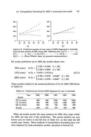
177. 6.4. Variable infectivity in chain binomial models 165
Table 6.8. Reed-Frost chain binomial probabilities for households of size four
Type of chain Probabilities* Expected values of probabilities*
4 4 a4
zq(3)/z(3)
43 3 4a6
(l-a) 4zq(b)zp(0)/z(6)
43 2 2 12a7
(l-a)2
12zq(6)zp(l)/z(S)
4 3 2 11 24a7
(l - a)3
24zq(6)zp(2)/z{9)
4 3 2 10 0 24a6
(l - a)4
24zq(5)zp(3)/z(9)
43 2 00 12a5
(l-a)4
2zq(4)zp(3)/z(S)
4 3 11 12a6
(l - a)3
12zq(5)zp(2)/z(S)
4 3 10 0 12a4
(l - a)3
(l - a2
) I2zq(3)zp(3)(l + q + 12z)/z(S)
4 3 0 0 4a3
(l - a)4
4zq(2)zp(3)/z(6)
4 2 2 6a6
(l - a)2
6zq(b)zp(l)/z{7)
4 2 11 12a5
(l - a)2
(l - a2
) I2zq(4)zp(2)(l + q+ 13z)/z(S)
4 2 10 0 12a4
(l - a)3
(l - a2
) 12*g(3)zp(3)(l + q + I2z)/z(8)
4 2 0 0 6a2
(l - a)2
(l - a2
)2
Qzq(l)zp(3)[76z2
+ (17 + 19q)z + (1 + q)2
)/z(7)
4 1 1 4a4
(l - a)3
4zq(3)zp(2)/z(6)
4 10 0 4a(l - a)3
(l - a3
) 4zq{0)zp(3)[3Sz2
+ (12 + 9q)z + (1 + q)2
]/z(7)
4 0 0 (I-a)4
zp(3)/z(3)
*See equation (6.4.5) for definition of p, q, z and zp(-).
data, and the Reed-Frost model where ay = ay
, to the data. The Reed-
Frost probabilities are shown in column 2 of Table 6.8. Both fits proved
adequate but not ideal, with that of the Reed-Frost model the better.
Greenwood (1949) had considered possible variations in a, while Bailey
(1975) showed that if a is a random variable with a beta distribution, re-
flecting the variable infectivity of households, then chain binomial models
could provide an improvedfitfor the Providence RI measles data (see Bailey,
1975, Chapter 14, pp. 254-260).
Dietz and Schenzle (1985) reviewed the history of household epidemic
statistics and considered the data of Heasman and Reid (1961) who had
obtained a = 0.886 for the probability of no contact in the Reed-Frost
model. Becker (1981) found a = 0.884, and Schenzle (1982), after pooling
some of the data (see Table 6.9, column 3), obtained a = 0.893. Schenzle
(1982), following Bailey (1975), also considered the case of a Reed-Frost
model in which a is a beta random variable, but did not provide any details;
we reproduce his figures in Table 6.9, without having full knowledge of his
method of fit.
We now sketch the treatment of Gani and Mansouri (1987), from which
paper further details can be obtained. Following Bailey (1975) and Section
4.3 above, we have for the Reed-Frost model
Piiia) = Pi{(X,Y)t+1 = (j,i-j) I (X,Y)t = (i,y)} = (*Vl - avy-iavi.
(6.4.2)

178. 166 6. Fitting Epidemic Data
Suppose that a (0 < a < 1) varies between households and follows the beta
distribution with density function
(a,6>0). (6.4.3)
B(a,b) ( a
' 6 >
Then, integrating Pij(ot) over all values of a gives
>3
da
(6.4.4)
We can simplify the notation by writing
zr(n) =
a -f- o
+ fcs) (0 < r < 1),
= i - q s =
a + b
z(n) = zi(n) = + ks),
(6.4.5)
thereby obtaining the formulae in column 3 of Table 6.8.
Table 6.9. Common cold data for households of size four with four model fits
Chain
Xt= 4 4
4 3 3
4 3 2 2
4 3 2 1 1
4 3 2 1 0 0
43 2 0 0
4 3 11
4 3 1 0 0
4 3 0 0
4 2 2
4 2 11
4 2 1 0 0
4 2 0 0
4 11
4 1 0 0
4 0 0
Total
X2
Observed
data
423
131
36
14
4
2
8
2
2
24
11
3
1
3
0
0
664
Reed-Frost
variable a
420.77
133.52
40.17
10.43
1.82
1.09
6.12
2.41
0.53
23.15
13.34
2.41
3.21
2.84
2.18
0.24
664.23
2.74
models
fixed a
405.2
147.1
45.3
10.5
1.4
0.8
6.0
1.7
0.3
25.6
12.7
1.7
2.0
2.5
1.1
0.1
664.0
9.1
Becker's
general model
403.9
147.3
45.6
10.7
1.4
0.8
6.2
1.6
0.3
26.9
12.2
1.6
1.8
3.7
0.0
0.1
664.1
9.5
Schenzle's
model*
420.9
133.4
40.1
10.4
1.8
1.1
6.1
2.4
0.5
23.1
13.4
2.4
3.2
2.8
2.0
0.2
663.8
5.8
* A Bailey-type variant of the Reed-Frost model; see text for detail.

179. 6.4. Variable infectivity in chain binomial models 167
We now estimate the parameters q and s, and test the goodness-of-fit of
the model. Prom the third column of Table 6.8 and the observed data in
column 2 of Table 6.9, we may write the log likelihood function of the chain
probabilities as
In L = C 4- 664 In q + 664 ln(q + s) + 663 n{q 4- 2s) + 661 ]n(q + 3s)
+ 230 ln(q 4- 4s) + 217 n(q + 5s) + 50 ]n(q + 6s) + 241 lnp
+ 110 ln(p + s) 4- 50 ln(p 4- 2s) 4-14 ln(p 4- 3s) + 5 ln(l 4- q 4- 12s)
4-11 ln(l 4- <? 4- 13s) + ln(76s2
4- [17 4- 19q]s 4- [14- # )
- 6641n(l + s) - 6641n(l 4- 2s) - 6641n(l 4- 3s) - 241 ln(l 4- 4s)
- 241 ln(l 4- 5s) - 241 ln(l 4- 6s) - 105 ln(l 4- 7s) - 80ln(l -f 8s)
-181n(l4-9s) (6.4.6)
for some constant C. Gani and Mansouri (1987) used the ZXMWD subrou-
tine of IMSL to minimize — In L, and found for the MLEs of q and s
q = 0.8887 ± 0.0114, s = 0.0223 ± 0.0222, (6.4.7)
the corresponding information matrix being
T (31747.4 -4727.7 ( .
1
= (-4727.7 8535.7 J ' ( 6 A 8 )
and variance-covariance matrix
_ / 0.3433 x 10~4
0.1901 x 10"4
, .
~ 0.1901 x 10~4
1.277 x 10"4
) ' [ }
They obtained as the corresponding estimates of a and b
a = 39.91, 6 = 4.999.
Based on the estimates (6.4.7) of q and s, and the expected probabilities
in column 3 of Table 6.8, the fitted values for the Reed-Frost model with
variable a were calculated (see Table 6.9, column 3). These were then
compared with columns 4-6 of Table 6.9 carried over from results of Becker
(1981) and Schenzle (1982).
To obtain chi-square goodness-of-fit statistics, all chains with fitted values
less than 5 were combined. For the Reed-Frost model with fixed a (column
4 of Table 6.9), Becker obtained 2
= 9.1 with 6 degrees of freedom (P-
value = 0.166). For Becker's general model (column 5 of Table 6.9), 2
= 9.5

180. 168 6. Fitting Epidemic Data
with 5 d.f. (P-value = 0.091). The Reed-Frost model with variable a gives
a closer fit: 2
= 2.74 with 5 d.f. (P-value = 0.728). Schenzle's variant is
likewise closer than the fixed a and Becker's model.
These results lend support to the hypothesis, originally made by Green-
wood (1949), that there is variation in the susceptibility to infection between
households. Bailey (1975) had already shown in his studies of the Provi-
dence RI measles data that both Greenwood and Reed-Frost models with
variable a provided improved fits. The present application to common cold
data arrives at a similar conclusion.
6.5 Incubation period of AIDS and the back-calculation method
At the end of Section 6.2, we mentioned that simple extrapolation fore-
casting had now been replaced by the back-projection or back-calculation
method as a means of predicting the number of HIV seropositives and AIDS
patients in a population. The models used in this method rely on the rela-
tion between HIV incidence in the time interval (s, s + ds) and the subse-
quent AIDS incidence in the time interval (t,t + dt) where t > s, following
an incubation period of length x whose distribution f(x) is assumed to be
known. This incubation period is defined as the time from the instant of
infection by HIV to the onset of AIDS, where the onset is evaluated in terms
of external clinical symptoms, or by a patient's T-4 cell count (also called
CD-4 count). When this count falls below a certain threshold, e.g. below
200/mm3
blood, say, then the patient is said to have AIDS. The expected
number a(t) dt of new cases of AIDS in (t, t + dt) is given by
a(t)= / I(s)f(t-s)ds
Jo
where I(s) ds is the number of HIV cases reported earlier in (s, s + ds). The
integrated form of this equation expresses the cumulative number A(t) of
AIDS cases to time t in terms of the distribution function F(t) = JQ f(u) du
of the AIDS incubation period, namely
A{t)= f F{t-s)I{s)ds. (6.5.1)
Jo
The distribution f(u) is usually assumed to be of Weibull or gamma type,
with an approximate mean of 10 years. On the basis of past HIV infection
curves, fitted parametrically or non-parametrically, one can project future
numbers of AIDS cases.

181. 6.5. Incubation period of AIDS and the back-calculation method 169
Equation (6.5.1) can be used in one of two ways:
(a) assuming I(s) and F(t) are known, one can calculate A(t); and
(b) assuming A(t) and F(t) are known, one can calculate I(s).
It should be noted that data on A(t) are far more reliable than data on /(s),
so that case (b) then allows a reasonable estimate of I(s) to be obtained. On
the other hand, for predictions of A{t), even an imperfect I(s) can prove
useful. The key in both cases is the distribution F(t) of the incubation
period, and we begin by considering this.
Several authors have studied the distribution of the incubation period,
relying on data from transfusion-associated AIDS patients, for whom the
date of initial HIV infection is known. There are for example early papers
by Lui, Lawrence et al. (1986) and Lui, Peterman et al. (1988) in which the
data are fitted by a Weibull distribution, with due allowance for truncation
at the reporting date (31 December 1984 for the earlier paper). Denoting
the 3-parameter Weibull distribution by
F(t; A, r, 6) = 1 - (t > 0 > 0), (6.5.2)
these authors estimated the parameters A, r and 6 from the data, and
concluded, on the basis of 83 adult individuals undergoing transfusions from
1978 to 1983, that the mean incubation period was 54 months = 4.5 yr, with
90% confidence bounds of 2.6 and 14.2 yr. The estimated Weibull density
function for this case is shown in Figure 6.6 below. We used the parameters
A = 0.000044 5, f = 2.51 and 6 = 2.5 months for this density function, and
our time axis is in months. The modal value of the density turns out to be
larger than in Lui, Lawrence et al. (1986).
0.02-
0.015-
0.01-
0.005 -
I
20
I
40
I
60 80
I
100
I
120
Figure 6.6. Estimated Weibull density function for the transfusion-
associated AIDS incubation period in months based on 83 adult patients.
(Based on Figure 2 of Lui, Lawrence et al. (1986).)

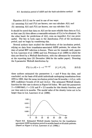
182. 170 6. Fitting Epidemic Data
Other authors have used different models for the distribution of the in-
cubation period, such as the gamma density function
Among these are Anderson and Medley (1988), who estimated values of
a = 2.7, A = O.lOyr"1
, hence a mean of 2.7/0.19 = 14.3 yr, based on
fitting a gamma distribution to data from England and Wales up to April
1988. They also fitted the 2-parameter Weibull distribution F(t p, /?) =
1 - e " ( ^ , obtaining {3 = 2.33, p = 0.12 yr"1
and a mean of 7.4yr (cf. the
parameters used for Figure 6.6, for the d.f. 1—exp (—[p(t — O')]P), which has
/? = f = 2.51,0' = 0.2yr, p = 12(0.000044 5)1
/251
= 0.221 yr"1
). Lawless
and Sun (1992) considered in addition a log logistic distribution function
( 6
" >
Each of these distributions for the incubation period provides an adequate
fit to various transfusion associated data sets. On the other hand, Bac-
chetti, Segal and Jewell (1992), who estimated the incubation distribution
from similar data on haemophiliacs using two different parametric mod-
els (including the Weibull distribution as a special case), concluded that
their analysis showed significant evidence against the Weibull distribution.
We would comment simply that fitting any particular distribution without
having a model-based rationale for doing so, provides no assurance of the
propriety of the chosen distribution.
An excellent survey of methods used in the estimation of the AIDS incu-
bation period, and the back-calculation method, may be found in Section 1
of Jewell, Dietz and Farewell's book (1992) on AIDS Epidemiology. Further
details are also available in some of the early papers (Brookmeyer and Gail,
1988; Centers for Disease Control, 1990; Brookmeyer, 1991; and Solomon
et al., 1991).
We now give some detail of the methods in Lui, Peterman et al. (1988) for
paediatric patients, as an example of the procedures commonly used. Their
data consisted of the incubation periods U of 32 patients (i = 1,..., 32) in
the period 1979-1984, while the AIDS diagnoses were made in the period
1982-1985. For patient i let Ri denote the number of months between trans-
fusion and 31 December 1985, Li the number of months between transfusion
and 1 January 1982 (the month of the first diagnosed case of AIDS). Then

183. 6.5. Incubation period of AIDS and the back-calculation method 171
assuming (6.5.2) holds, the likelihood of the observed data can be written
as
L
=
where ^ = 1 if the critical transfusion date for i was before January 1982,
Si = 0 otherwise. Thus, when 8i — 1,
F{Ri) - F(Li) = e - A
( L
- - ^ r
- e~x
^-e)r
= Pr{Lt <U<
and when 8i — 0,
The maximum likelihood estimates of r and A can now be obtained, assum-
ing the value 6 = 3 months which is found to maximize L for the values of
r and A derived from the equations
Writing these out in full detail, we have
a i n L 3 2 **
32
32 32
E ln
(^-«) -E A
«< -°r ^ -
—OiAylji — uj LllyL/i — uJQ v
' -- Ayiii — u) in^XL^ — I
The results obtained were f = 1.418, A = 0.00856 with 0 = 3, giving a
mean incubation period of 29 months or 2.4 yr with an approximate 90%
confidence interval of 18 to 86 months. The mean is smaller than the equiv-
alent mean for adults (4.5 yr) quoted earlier. The estimated Weibull density
function for the 32 paediatric patients is given in Figure 6.7, with the time
axis in months as before. Note that this differs considerably from Figure
6.6, both in its range and its shape.

184. 172 6. Fitting Epidemic Data
0.025 -
0.02-
0.015 -
0.01-
0.005 -
0-
0 20 40
I
60
I
80 100
Figure 6.7. Estimated Weibull density function for the AIDS incubation
period in months based on 32 paediatric patients. (Based on data in text
from Lui, Peterman et al. (1988).)
An alternative approach is to use death or birth-and-death processes for
modelling the associated T-4 cell count process as in Gani (1991) and Rossi
(1991). Whatever model is used, one may assume that the distribution
function F(t) of the incubation period of AIDS is adequately estimated.
We now proceed with the back-calculation method itself.
6.5.1 The distribution of the AIDS incubation period
Solomon et al. (1991) used AIDS data for Australia from 1982 to 1990 to
reconstruct HIV prevalence; these data are reproduced in Table 6.10 and
thereby bring Table 6.3 up to date to 1990, including revisions of the data
given previously.
Table 6.10. Quarterly AIDS diagnoses in Australia, 1982-1990
Year
Quarter
1982
1983
1984
1985
1986
1987
1988
1989
1990
0
1
26
42
86
112
142
150
1
6
37
51
96
112
121
131
2
16
29
63
87
143
153
167
1
3
23
30
70
102
155
152
143
Using the 2-parameter Weibull distribution in the form
(6.5.7)

185. 6.5. Incubation period of AIDS and the back-calculation method 173
with r = 2.55 and A = 0.002078yr~255
= (0.0887)V2.55yr-2.55 for t h e
AIDS incubation period distribution, and adopting a parametric approach
in which the HIV infection curve is assumed to be either
(a) quadratic exponential, I(t) = aoexp(ait — a2t2
), or
(b) linear logistic, I(t) = (60 + bit)/(I + e62
~M
),
then the AIDS diagnoses in a particular quarter (^,£7+1) are predicted by
A(tj+i) - A(tj) = f J+1
I(s)F(t -s)ds (j = 0,..., 33).
Here the increments in A(-) are known from Table 6.10, F(t) is given by
(6.5.7) with (r, A) = (2.55,0.002078), and I(t) has one of the two para-
metric forms mentioned; it is, of course, possible to reconstruct I(t) non-
parametrically.
Given these conditions, assuming the epidemic to have begun in 1981,
Solomon et ai. (1991) obtained the following estimates of Jy+
I(s)ds for
the years (y,y + 1) in the period 1981-1990.
Table 6.11. Estimated annual HIV infection incidence in Australia
Model
(a) Quadratic
exponential
(b) Linear
logistic
Year
(i)
(ii)
0)
(ii)
1981
34
34
62
62
'82
912
912
678
678
'83
4046
4046
4032
4032
'84
4380
4380
5522
5690
'85
1160
1374
1000
'86
73
1000
1000
'87
1
1000
1000
'88
1000
1000
'89
1000
1000
'90
1000
1000
The values at i) for both the quadratic exponential and linear logistic curves
are calculated without adjustment, while at ii) they include various adjust-
ments, such as an allocation of 1000 new HIV cases annually from 1986 in
A and 1985 in B, or the effects of various treatments, in order to achieve
greater realism. From these scenarios, HIV infection curves can be recon-
structed under different assumptions.
These HIV infection curves can then be used to make short-term projec-
tions of new AIDS diagnoses from (6.5.1). Table 6.12 sets out these for the
years 1991-1995 for Australia as given in Solomon et ai. (1991).
Table 6.12. Estimated annual HIV infection incidence in Australia
Year 1991 '92 '93 '94 '95
Quadratic exponential I(t) 765 830 863 863 831
Linear logistic I{t) 756 816 844 840 804
Note: No actual numbers are available for comparison

186. 174 6. Fitting Epidemic Data
6.6 Exercises and Complements to Chapter 6
6.1 As a setting for a continuous time analogue of (6.1.2) and (6.1.3), let X(t),
Y(t), Z(t) denote the number of susceptibles, the (analogue of the) number
of infectives at time t, and the number of deaths by time t. Develop the
following relations:
rJo
= -0X(t)Y(t), i.e. ±
v(u)du + J <p(t~u)dX(u),
where X/J(U) denotes the probability that an infected individual is still in-
fectious (and mixing in the population) time u later, and Kip(u)du is the
probability that an infected individual dies in the interval (u,u + du) after
infection. Observe that, from an algorithmic viewpoint, the discrete time
model is easily implemented, but not so the continuous time model.
6.2 Table 1.6 presents data of En'ko (1889) recording the daily numbers of
measles cases for several years from records at the Smolnyi Institutions. Find
estimates of the variance of the dates of identification of cases within each
generation, (a) for each year as tabulated, (b) for the pooled data. Is there
any evidence for a model like s^U) = a
m + 0mj, for m = a, b according
as data are from (a) or (b) and j = generation number. How would you
interpret a& = 2aa, 0b = Pa ?
6.3 Consider a chain binomial model in which the probability pt of pairwise in-
fection is no longer constant but is monotonically non-increasing in t. This
can reflect the propensity of individuals who are more gregarious or more
infectious or more susceptible, to be infected ahead of others. Investigate the
estimation of {pt} and the fit of such models to data like Aycock's measles
epidemic (Table 1.5) or En'ko's data (Tables 1.6 and 4.1).
Hemark: This discrete time model attempts to reproduce the effects of het-
erogeneous mixing or infectivity and susceptibility as done for continuous
time models in Cane and McNamee (1982) and Daley, Gani and Yakowitz
(2000).

187. 7
The Control of Epidemics
One of the purposes of modelling epidemics is to provide a rational basis for
policies designed to control the spread of a disease. This aim was already
evident in Macdonald's pioneering work on malaria. In his Presidential
address to the Royal Society of Tropical Medicine and Hygiene (Macdonald,
1965), he referred to the development of a prevention strategy for epidemics,
malaria in particular, stating that
there is only one way of doing this—through a working model... made
by assembling all we know, or more aptly, all that we believe to be sig-
nificant, of the factors involved in transmission ... in a form describable
in mathematical terms.
A major contribution of Macdonald compared with his predecessors (he
mentions Farr, Brownlee, Ross, Lotka, Kermack and McKendrick) was to
pursue this approach to its
logical conclusion—of final interpretation of mathematical reasoning
into non-mathematical explanations of epidemiological happenings such
as could be readily understood by most practising epidemiologists.
In this spirit we consider three models for epidemics to illustrate possible
prevention policies of control by (a) education, (b) immunization, and (c)
screening and quarantine. We could add that modelling is of vital impor-
tance in evaluating the likely effects of spreading a disease deliberately as a
means of biological control, as with myxomatosis or the calicivirus to reduce
the rabbit population in Australia.
Often the data available to decision makers are inadequate, as for example
in the case of HIV/AIDS in Africa or South East Asia. Yet policies need
to be formulated, if only on the basis of rough qualitative measures. One
175

188. 176 7. The Control of Epidemics
may, for example, need to know the likely effects of spending funds on two
alternative policies, or the optimal method of immunizing a population.
Here, exact models may not be easy to formulate, though one usually tries to
make all modelling as realistic as possible. Accurate data may be impossible
to obtain, but one should always be in a position to minimize the cost of
a policy or to compare the effects of policy A against those of policy B,
however approximately. Examination of the control methods discussed in
this chapter shows that they use and extend the simple models discussed in
previous chapters.
When a policy depends only on a single variable, it is relatively easy to
minimize the cost. If two policies are to be compared, one can examine
their respective costs and choose the cheaper policy. Alternatively, if the
criterion is not cost, one can rank the policies with respect to the criterion
selected.
The control methods we describe in this chapter can be understood in
terms of the general epidemic model of Chapters 2 and 3, with pairwise
transmission rate (3 and removal rate 7, or of more complex models that
include this as the simplest case. We present strategies aimed at one or
more of the following results:
(a) depressing the number of susceptibles in the population, and, where
possible, to below the threshold level p = 7//? described earlier in the
Kermack-McKendrick criticality theorem (Theorem 2.3.1 above);
(b) accelerating the rate of removal of infectives to reduce their mixing
with the population of susceptibles (i.e. increasing 7, hence p also);
(c) lowering the pairwise rate of infectious contact between infectives and
susceptibles (i.e. decreasing /?, thereby increasing p).
For example, immunizing some or all of the population reduces the initial
number XQ of susceptibles; operating a screening program or raising public
awareness of higher disease prevalence may raise 7 or lower (5 (or both);
discouraging the assembly of large crowds reduces /?.
7.1 Control by education
The AIDS epidemic has spread rapidly throughout the world. But its ef-
fect has been more limited in countries where a campaign for information
and education has been sponsored by the state, or by a foundation, as for
example in Switzerland.
In February 1987 a 'STOP-AIDS' advertising campaign was launched by
the Swiss AIDS Foundation to provide the population with detailed knowl-
edge of the AIDS infection and its spread, and to discourage risk-prone

189. 7.1. Control by education 177
Table 7.1. Annual expected increase 32 000(1 — m — pr)na
in the number of infectives
n
a
0.05
0.10
0.15
r
1
1372
2744
4116
Before advertising
(m =
= 0.25
3
4116
8232
12348
= 0.08,
5
6860
13729
20580
p = 0.25)
r = 0.50
1 3
1272 3816
2544 7632
3816 11448
5
6360
12720
19080
r
1
1148
2296
3444
After advertising
(m =
- = 0.25
3
3444
6888
10332
0.17,
5
5740
11480
17220
p = 0.45)
r = 0.50
1 3
968 2904
1936 5808
2904 8712
5
4840
9680
14520
behaviour by recommending (a) the use of condoms in sexual contacts with
multiple or casual partners, (b) mutual faithfulness between sexual partners,
and (c) the use of clean needles in drug usage (i.e. no exchanges between
users).
It emerged that between January and October 1987, the number of oc-
casional sexual contacts of those aged 17-30 years in Switzerland declined
from 18 to 14% of the population, and among these the number always us-
ing condoms in sexual contacts increased from 8 to 17%, while those using
them sometimes increased from 25 to 45%. The number of condoms (about
9.2 million) placed on the market in this nine-month period increased about
60% over the same period in 1986 (see Hausser et al., 1988).
We can calculate roughly the effect of such greater sexual caution on
the development of an AIDS epidemic as follows, using illustrative numbers
for the land of Erehwemos with a population of 6.4 million where before
a campaign like STOP-AIDS begins, we assume that the number of HIV
carriers is 0.5% or 32,000 infectives. If on average each infective has n
sexual partners in a year, with each of these partners being infected with
probability a, where 0.05 < a < 0.15, then the number of new infectives to
be expected would be about 32000na. If as a result of a STOP-AIDS type
campaign a proportion m < 1 of these infectives always use condoms, and
a further proportion p < 1 — m use condoms for a proportion r of the time,
then the number of new infectives expected in a year would be about
32000(1 -m-pr)na. (7.1.1)
This assumes that condoms provide total protection from HIV infection.
Table 7.1 lists the number of new infectives expected in a year for different
values of the proportions m of regular and p of occasional condom users,
the latter using them a proportion r of the time. The values of m and p in
the table are assumed to be similar to those reported in Switzerland. The
infection rate is set at 0.05(0.05)0.15, and the number of sexual partners

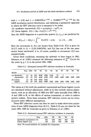
190. 178 7. The Control of Epidemics
n == 1, 3 or 5. Depending also on whether r = 0.25 or 0.50, the number
of new infectives computed by the model would decline between 16.3% and
23.9%. This indicates the extent to which a STOP-AIDS type campaign
could be expected to modify the course of the epidemic.
One could imagine that a government might wish to minimize the total
cost C of (a) the annual expenditure y on pamphlets, advertisements and
other educational material, and (b) the cost of medical treatment of HIV
patients, each of whom requires the sum c per annum. The total expenditure
C at the end of the year, starting with N HIV seropositives, would be
C = [N + N(l - m - pr)na]c + y. (7.1.2)
Suppose now that plausible equations for m and p are
m = I ( l - e - f c
» ) , p = | ( l - e - * » ) , (7.1.3)
where k > 0 is some constant, and the maximum proportions of regular and
occasional condom users, whatever sum y is spent on education, are | and
| respectively. Then the expression for C at (7.1.2) becomes
C = Nc + JVnac[f(l - r) + {l + 2r)e~ky
} + y. (7.1.4)
This function is concave in y, so differentiation yields an equation for the
value of y giving the least cost C, with solution
y = In (k(l + 2r)Nnac). (7.1.5)
As an example, suppose we take r = 0.25, N = 32000, a = 0.10 and
n = 3, while c = 1 is the financial unit. Then y = k~* ln(4800fc). Depending
on the value of h, the value of y rises from 0 to a maximum of 1765.8 before
decreasing to 0 as k —> oo, as shown in Table 7.2 and Figure 7.1. In
the optimal scenario, the budget y for educational material will be 1765.8,
leading to a minimal cost C = 44451.9 where y/C = 3.97%. Choosing some
smaller y, say y = 61.7 for k = 0.1, yields minimal cost C = 36895.1 so
that y/C = 0.17%.
Table 7.2. Values ofy for different k
0.01 0.1 1.0 10
-4.61 -2.30 0 2.30
307.12 61.74 8.48 1.08
k
lnfc
y
0.0002083
-8.48
0
0.0003
-8.11
1215.48
0.000566309
-7.48
1765.82
0.001
-6.91
1568.62

191. 7.2. Control by immunization 179
1500-
1000-
500-
0
Figure 7.1. Graph of y as a function of In k.
While there is no claim that these are realistic figures, the calculations
we have given indicate the type of decision that policy makers can attempt
to make in the allocation of funds. In this example, spending on education
a sum that is approximately 4% of the cost of medical treatment, results in
a minimal cost C.
A recent paper of Kaplan (1995) on the merits of needle exchange for
intravenous drug users provides an alternative example of HIV control by
education. O'Neill (1995) has also studied epidemic models in which be-
havioural change plays a role.
7.2 Control by immunization
Immunization has long been used as a method for controlling the spread
of an epidemic; in the case of smallpox, a worldwide vaccination campaign
succeeded in eradicating the disease totally (see Fenner et ai., 1988). The
fact that parents are sometimes lax in ensuring that their children are im-
munized against preventable diseases like measles and poliomyelitis for ex-
ample, has resulted in their random recurrence. Accounts of animal and
human immunization schemes may be found in Knox (1980), Dietz (1981)
and Anderson (1982), among other authors. Readers should, however, note
the cautionary remarks on Knox and Dietz's work in Anderson and May
(1991, pp. 152-153).
In considering immunization as a technique for controlling the spread of
a disease, at least two policy questions arise, both subsumed in the pursuit
of maximum effect with minimum effort:
(a) how widespread can (or, should) the immunization be, and
(b) which susceptibles should be immunized for this effort to produce the
best effect (e.g. should individuals be immunized at random, or should
groups such as schools or families be targeted)?

192. 180 7. The Control of Epidemics
These questions involve us in detailed modelling of the population where the
immunization takes place, and in estimating its effect given some description
of how the disease spreads. If infection spreads homogeneously through the
population then question (b) is void.
Any quasi-realistic description of the spread of contagious infection usu-
ally requires recognition that the population in which the process occurs is
inhomogeneous. Yet even when the population is subdivided into groups of
individuals belonging to different strata (however defined), those in a given
stratum are assumed to mix homogeneously amongst themselves, and to
behave similarly towards individuals of other strata. In other words, ho-
mogeneity is not entirely dispensed with, for it is this very similarity that
underlies the statistical approach. As in Section 3.5, we use the neutral term
'stratum' to describe such sub-populations within which individuals are re-
garded as identical apart from their disease status, noting that it may cover
spatial variability, or distinct social behaviour, for example. Anderson and
May (1991, Chapter 12) describe an optimal immunization strategy within
a spatially heterogeneous population; Becker and Dietz (1995, 1996) have
considered a population consisting of a number of smaller units (households,
clubs or schools), and computed the effects of different strategies determined
by the characteristics of these units. The four particular strategies they dis-
cussed were
(i) random immunization of individuals;
(ii) households chosen at random and all their members immunized;
(iii) preferential selection of large households for immunization;
(iv) immunization of a fixed fraction of members in every household.
Suppose for the moment that immunization is to be administered uni-
formly and at random in a population that is susceptible to a disease which
is characterized by a Basic Reproduction Ratio Ro (see Section 3.5). Recall
that the threshold criterion can be stated in terms of this as
the disease can spread if Ro > 1, whereas it cannot if Ro < 1. (7.2.1)
Then, a result dating back at least to Gordon Smith (1964, Figure 3) states
that v*, the minimum fraction of the population that should be immunized
so as to prevent a major outbreak, is given by
v* = 1 - l/ifo. (7.2.2)
If immunization is carried out randomly and uniformly in a stratified pop-
ulation, then equation (7.2.2), first established for a single homogeneously

193. 7.2. Control by immunization 181
mixing population, also holds for stratified populations with the general defi-
nition of Ft®. To see this, recall that Ro is defined as the dominant eigenvalue
of a linear mapping between strata determined by the mean number ra^
of j-stratum infectives produced by an z-stratum infective during its entire
period of infectivity. Now a random uniform immunization programme at
level v reduces the expected number of susceptibles uniformly by the con-
stant factor (1 — v). The m^ are therefore reduced similarly, and thus all
eigenvalues are reduced by the same factor. In particular the Reproduction
Ratio is (1 — v)Ro, and when (7.2.2) holds, this equals the critical level of
unity (see (7.2.1)).
That this relation fails to provide the optimum immunization strategy in a
genuinely heterogeneous population, where pairwise infection transmission
rates (3 within groups are typically higher than between groups, is intu-
itively understandable (Anderson and May (1991), p. 307). Immunizing the
same fraction in all strata results in relatively too many immunes in small
groups and too few in large groups; the deficit in the latter is not made up
by the excess in the former because the overall rate of infectious contacts
is quadratic in the group size. Thus a uniform immunization rate, to be
effective in the population as a whole, must produce more immunes than
would be needed for uniform immunity within the separate strata. Using a
deterministic model, Anderson and May showed that, if the pairwise infec-
tion rates (3ij for an z-stratum infective to transmit the disease to a specified
j-stratum susceptible are fiij = (3H OT /3C depending only on whether i = j
or i 7^ j respectively, then the optimal policy (i.e. requiring the minimum
total amount of immunization) is such that the non-immunized suscepti-
ble numbers in each stratum are identical. Again, this is understandable,
for such an immunization program reduces the susceptible populations to a
collection of identical sub-population units.
In more detail and in a stochastic setting, consider a population of m
strata with Ni susceptibles, i = 1,... ,ra, as in Example 3.5.1, in which
the pairwise infectious contact rates are (3H within each stratum and (3c
between strata. We saw at (3.5.14) (recall also Exercise 3.10) that when no
Ni is small,
Ro > P" + ("y
1
)frl*, (7.2.3)
where N = Y^iLi Ni/m; equality holds, when (3H ¥" Pc, if and only if all Ni
are identical. Suppose that as a result of an immunization programme the
Ni susceptibles are reduced to TV*, say. Then the resulting Reproduction
Ratio RQ, say, would satisfy (7.2.3) with N replaced by ~N*, and the equality

194. 182 7. The Control of Epidemics
would now hold if and only if all N* are equal. Consequently, among those
immunization programmes that reduce RQ to RQ = 1, the programme re-
quiring the smallest number of people to be immunized (i.e. the programme
for which m(N - ~N*) is least), is the one for which each Ni is reduced to
This analysis depends on none of the Ni being small, a condition which
is not generally met when each stratum is a household; in this case an
alternative setting is needed, such as was discussed in Example 3.5.2. There
we showed that when (3H > 7, Ro ~ (A + V'A2
+ 4B), where
Here ^4, but not 5, is independent of the detailed household structure.
Suppose that under an immunization strategy, the Ni are reduced to AT*,
so that A, B and Ro reduce to A*, B* and RQ respectively, where these are
given by
B* =
l
^=* * v l
Y,i=iNi{Ni-l) ' (7.2.6)
Inspection of the expression for B* shows that it is a convex increasing
function of each N*. Hence a maximal reduction in R$ is achieved for a
given overall reduction AN = £2=1 W""-^*) m t n e
number of susceptibles,
when max; Ni is reduced maximally subject to this given total reduction.
Thus the conclusion immediately above (7.2.4) continues to hold in this
changed setting.
Specifically, given the number AN of susceptibles to be immunized, RQ
is reduced maximally by finding d for which N* = min(ATi,rf) and AN =
Y!j=i(N
i - d)+> w
*th
0 < N* < N^ This is a discrete analogue of the
continuous variable result of Anderson and May (1991, Chapter 12 and
Appendix G) referred to above (7.2.3). In fact, unless d is an integer, to
attain the optimum exactly we must further adjust the N? for those i for
which 0 < d — N? < 1 so that all the adjusted N* are integers.
Administratively, this optimal policy may not be as convenient as the
uniform fraction (i.e. strategy (i)), or the targeting of specific households
(either (ii) or (iii)), and so may prove more costly. But knowing the na-
ture of an optimal strategy, provides a rational basis for the assessment of

195. 7.2. Control by immunization 183
Table 7.3. Values of the reproduction ratio and immunization fractions for
different strategies in the case /3H ^> 7
k
™k
R*
^opt
*>unif
Kv
all/none
1
300
0.4998
0.5305
0.7435
0.1499
0.8592
2
400
3
200
4
75
Quasi-optimal strategy
1.3626
0.2019
0.3007
1.7439
0.0610
0.1050
1.8933
0.0141
0.0283
All-or-none in households > k
0.9640
0.4836
1.5106
0.2019
1.8027
0.0610
5
20
1.9379
0.0023
0.0054
1.9114
0.0141
6
5
1.9485
0.0000
0.0000
1.9485
0.0000
other policies. For example, if instead one were to immunize the largest
households completely, how much more immunization would be needed?
We discuss such questions in Example 7.2.1 and Exercises 7.1 and 7.2.
Example 7.2.1. Consider a population of m = 1000 households consisting
of rik households with k susceptibles (k = 1,... ,6) as shown in Table 7.3;
let 7 = 1, (5c — 0.0005. Suppose first that /?# » 7 so that all the analysis of
Example 3.5.2 is applicable. From equation (3.5.20) the Basic Reproduction
Ratio .Ro of the population equals 1.9485 as shown in the last column.
The rest of the entries in the table show the effects of three immunization
strategies.
The effect of the Quasi-optimal strategy, when immunization is carried
out to reduce all households to a maximum of j susceptibles, is shown
via the reproduction ratio RQ that would then be realized. This entails
immunizing a fraction vopt = Ylk>j(^ ~ J)n
k/ Ylk>i ^nk
°^ ^ne
population;
of course, vopt < fUnif = 1 — RQ/RO, the fraction needing immunization
under a random strategy to reduce the reproduction ratio by the same
amount.
Consider next the effect of an all-or-none strategy in which all members
in every household of more than k members are immunized (strategy (ill)).
Then the reproduction ratio R'o and fraction immunized ^aii/none a r e a s
shown. The population numbers in the households were chosen so as to
make some of the vaii/none fractions coincide with fractions vopt under the
quasi-optimal strategy but for smaller k. Observe that the ratios under
the quasi-optimal strategy are smaller than the ratios under the all-or-none
strategy when ^li/none = vopt.
We can draw at least two conclusions from this table, for this particular
distribution of households. First, to reduce the value of the reproduction
ratio to below 1, requires the immunization of about 50% more individ-

196. 184 7. The Control of Epidemics
Table 7.4. Values of the reproduction ratio and immunization fractions for
different strategies in the case /3H = 0.27
k
nk
R*
^opt
Vunif
R'o
^all/none
1
300
0.4998
0.5305
0.6194
0.1499
0.8592
2
400
3
200
4
75
Quasi-optimal strategy
0.9697
0.2019
0.2615
1.1933
0.0610
0.0912
1.2802
0.0141
0.0250
All-or-none in households > k
0.6518
0.4836
1.0235
0.2019
1.2184
0.0610
5
20
1.3065
0.0023
0.0050
1.2892
0.0141
6
5
1.3131
0.0000
0.0000
1.3131
0.0000
uals under a random strategy than under the optimal one. Second, the
all-or-none strategy is marginally more efficient than the random strategy.
Strategies (ii) and (iv) are considered in Exercises 7.1 and 7.2.
Suppose now that /3# ^> 7 does not hold. The analysis we have given
must then be reworked starting from the matrix M at (3.5.18) and finding
its eigenvalue of largest modulus, much as in the concluding paragraph of
Section 3.5. We illustrate this approach in the context of Example 7.2.1 ex-
cept that now f3H = O.27 while the other parameter values are unchanged.
We computed the dominant eigenvalue by reduction of M to upper Hessen-
berg form via Gaussian elimination and use of the QR algorithm as in Press
et al. (1987, Chapter 11). This leads to Table 7.4 in place of Table 7.3.
Qualitatively, what is an optimal immunization strategy for an epidemic
that may spread in a community of households, for which the conditions
justifying the approximations do not hold? Intuitively, since the optimal
strategy described earlier is a function of the graph-theoretic structure of
the infectious path of the disease, then, assuming the same homogeneity
within households and the same infectivity relation between households,
we would expect the same strategy to remain optimal. In other words, the
quantitative details may change, but the qualitative principle would remain.
7.3 Control by screening and quarantine
A third method of controlling the spread of a disease is by screening sus-
pected infectives and quarantining those who are thought to pose a risk.
This is a procedure often adopted in countries free of malaria (e.g. Aus-
tralia) when a returning tourist is suspected of carrying the disease. In
California, prisoners known to be HIV seropositive (i.e. HIV+) are interned
in a separate correctional facility at Vacaville, but in general HIV screening

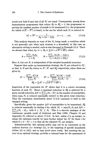
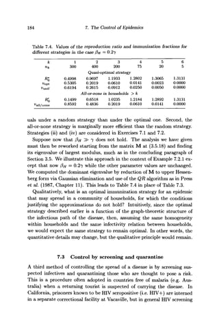
197. November 1985
October
October
October
October
October
1986
1987
1988
1989
1990
November 1992
766
1232
1964
3136
5411
6985
11565
7.3. Control by screening and quarantine 185
Table 7.5. Numbers of AIDS cases among US correctional inmates, 1985-1992
Survey period Number of cases Per cent increase from preceding survey
61%
59%
60%
72%
29%
66% [= 29% p.a.]
Source: Thomas and Moerings (1994), p. 139.
is not compulsory. The fact that HIV is more prevalent in prisons than
in the community at large, suggests that HIV may spread more rapidly in
confinement than in the free community (see Exercise 7.2).
HIV is spread in prisons by sexual contacts and by needle sharing among
intravenous drug users (Brewer et al. 1988). The US Department of Justice
(1993) reports that there were 11 500 known cases of AIDS in Federal prisons
for the five months from November 1992 to May 1993, with an average
growth of over 50% annually during the past several years (see Table 7.5).
This was considerably greater than the rate of increase in the total number
of prisoners (roughly, 75% between 1985 and 1992), and represented an
incidence rate of over 1% (cf. less than 0.1% in the wider population then).
Thomas and Moerings's book (1994) has documented worldwide concern
about the spread of HIV/AIDS in prisons.
Blumberg and Langston (1991) raised the question of mandatory HIV
testing of prisoners on entry into jail, but such a procedure is not currently
acceptable. However, voluntary reporting or testing for HIV is possible
(Stevens, 1993; see also Hsieh, 1991), and both medical and educational
help then becomes available to HIV4- prisoners; Siegal et al. (1993) state
that HIV-f prisoners who do not report their status do not receive medical
help. Hsieh (1991) considered a model of HIV screening that incorporates
the quarantine of infectives.
We consider in turn models for a single isolated prison, and for a prison
interacting with the outside world. Then in Section 7.3.3, we discuss a
screening and quarantine procedure for which the overall medical costs over
a fixed period of time T, including costs of treating undiagnosed HIV-h
prisoners, are minimized.
While only deterministic models are used here, their stochastic equiva-
lents can also be analysed (see Yakowitz, Gani and Blount (1996), Gani,
Yakowitz and Blount (1997) for details, and Section 4.4 above for a related
model).

198. 186 7. The Control of Epidemics
7.3.1 The single prison model
Suppose that a prison containing N inmates, allows a simultaneous inflow
and outflow of n < N prisoners at time t (t — 0,1,.. .), after which there
are yt prisoners who are HIV-f and N — yt susceptibles. During the interval
(t, t -h 1), which we take to be relatively short so that yt does not vary
greatly in it, assume that homogeneous mixing occurs with an infection rate
/?, so that {3yt(N — yt) new infectives are produced. This is a discrete time
approximation based on the continuous time simple epidemic; for details
see Bailey (1975, Chapter 5) or Section 6.1 above (Daley and Gani (1999a)
discuss another model analogous to a simple epidemic). Thus at time t +1—
there are
yt)) (7.3.1)
infectives. In the outflow of n = rN prisoners at time t -f 1, there are
= ryt[l + 0(N - yt) (7.3.2)
infectives, and amongst the inflow of n new prisoners we can expect a pro-
portion fit to be infectives, where 0 < nt < 1, so at time t -f 1-f there
are
(1 - r)yt[l + 0{N - yt)] = /(yt,Mt) (7.3.3)
infectives amongst the N prisoners.
Are there stable scenarios for this model? We could ask whether a sta-
ble regime is reached starting from t/o infectives at time 0-f under the as-
sumption that ^t — M (a
^ *)•T° this end we examine the transformation
V *-»•fiy,^) f°r an
Y fixed points lying in [0, AT]. Observe that the function
g(y) = f(y, /i) — y is concave, with #(0) = rtfi > 0 and g(N) = n(/x — 1) < 0
under our assumptions on fi. Thus, a unique stable scenario yt = ys (all t)
exists, namely
_ (1 + (3N)(1 - r) - 1 + ^[(1 + 0N)(1 - r) - I]2
+ 4n/i/?(l - r)
Vs
~ 2)9(1 - r)
0(N -n)-r+ y/[P(N - n) - r]2
+ 4/xr/?(7V - n)
~ 2/3(1 - r) *
(7.3.4)
In the limiting case ji = 0, y3 = 0 is also a fixed point and further
argument is needed to decide which of these roots of g(ys) = 0 equals
Hindoo yt. The matter is easily decided: equation (7.3.4) always represents
the larger root, and is zero (hence, the only root in [0, AT]) if and only if

199. 7.3. Control by screening and quarantine 187
Table 7.6. Stable infective sizes in the single prison model for different n, fi, j3N
n
25
50
0.01
0.005
0.01
0.005
0.0
5.0
2.5
5.0
2.5
0.05
39.8
25.4
9.0
4.5
0.075
160.1
154.8
14.5
7.5
0.1
242.3
239.6
31.8
18.7
0.125
293.1
291.3
82.5
71.2
0.15
327.2
325.9
142.6
136.4
/3N
0.2
370.2
369.3
228.3
225.3
0.25
396.1
395.4
281.7
279.8
0.5
448.0
447.7
390.3
389.6
5
494.8
494.8
489.0
489.0
(1 -f /3N)(1 — r) < 1. In other words, (7.3.4) always gives the required root:
when fji = 0 it simplifies to
0 H/3N <r/(l-r),
N — r/[/3(l — r)] otherwise.
(7.3.5)
We interpret this equation as indicating that infection is contained to small
levels within the prison if the former case holds, i.e. if n > f3N2
/(l + f3N).
Example 7.3.1. Suppose that N = 500. Table 7.6 indicates the stable
values ys under a range of values for (3 for n = 25 and 50, and /x = 0.01
and 0.005. The time taken to attain these stable values depends on both
the initial infection intensity y0 and the contact rate /3 (see Exercise 7.3).
Note that when j3N exceeds the threshold r/(l — r) the endemic level rises
appreciably above the endemic level // of the new prisoners, though the
threshold does depend on interplay of all of /i, f3N and n. For f3N below
the threshold, ys « nfi/[r - 0N(1 - r)], « fiN for /? -+ 0.
7.3.2 Interaction of a prison with the outside world
Consider a city of fixed population size M with Yt infectives at time t =
0,1,..., in which there is a single prison with N inmates of whom yt are
infectives. We make the same assumptions as in the previous section con-
cerning the prison, so that in (£, t + 1) there are /3yt(N — yt) new prison
infectives. The same proportion of infectives leaves as before.
For the city population, homogeneous mixing and an infectivity rate /?0
per susceptible-infective pair produces /30Yt(M - Yt) new infectives. Sup-
pose also that deaths occur at rate 7, and that the number of births, all
healthy, equals the number of deaths, thus keeping the city population size
constant. Then at time t + 1—, before exchange with the prison occurs, the
city has
(l~j)Yt+p0Yt(M-Yt)

200. 188 7. The Control of Epidemics
infectives, so with r = n/JV, R = n/M,
yt + 1 - (l - fl)Yt[i - 7 + A)(M - ^t)] + n/t[i + /?(# - yt)] = h{Yt,yt),
yt+l = RYt[l - 7 + /?o(M - Yt)} + (1 - r)i/t[l 4- /3(JV - y*)] = /2(*t, Vt).
(7.3.6)
Write f{Y,y) for the vector-valued function (/i(Y,i/), f2(Y,y)). For a real-
istic model we require that for (V, y) in the rectangle [0, M] x [0, AT], /(Y, y)
should also lie within the rectangle. Since / is continuous, and the rectangle
is a compact set, there is at least one fixed point (Ys,ys) = f(Ys,ys) which
we interpret as a vector of stable values for Y and y. Then (Ya,y8) satisfies
(Ys _ ((l-fl)[l-7 + A>(M-n)] r[l + (3(N-ys)} ) (Ys
U J " I i ? [ l - 7 + A ) ( M - r s ) ] ( 1 - r ) [ l + / ? ( # - y , ) ] J { y s )
(7.3.7)
Addition of these two equations gives
Y.+y.= Ya[l - 7 + A)(M - Y.) + ys[l + /J(iV - y.)], (7.3.8)
and hence
(3OYS(M - Y.) + Pys{N - ys) =7 r s . (7.3.9)
Equivalently, the number of new infectives in (t,t + 1) equals the number
of infectives removed in (£, £ + 1). Substitution in (7.3.7) so as to eliminate
one or other of the quadratic terms yields
rys = R(l - 7)YS + (1 - R - r)(3ys(N - ys)
(l-r)jYs-(l-R-r)(30Ys(M-Ys),
showing that (0,0) and (M, N) are always fixed points, and that they are
the only fixed points when 7 = 0, i.e. when the city population has no births
and deaths.
Equation (7.3.9) shows that for the disease to be confined to a small
number, eM say, of the city population, the various parameters must sat-
isfy both (30M(l—e) < 7, i.e. the infection rate /3o must lie below a threshold
level determined by the relative removal rate 7/M, and the endemic infec-
tion level in prison ys must likewise be contained by a function, namely
0ys{N-ys) < (<y-(3oM)eM. Ideally, having (3 < 4(7-/3oM)eM/N2
would
contain the incidence in the city population irrespective of the incidence
rate in prison. See also Exercise 7.4.
Rewrite (7.3.7) as 0 = gi(Ys,ys) = fi(Ya,y8) - Ya, and 0 = g2(Ys,ys) =
f2(Ysyys) — ys. For given z/, <7i(Y, y) is concave in Y, with stationary point
Y(y) equal to
v , ^ - A + yM + 4fl>(l - R)ry[ + (3(N - y)}
Y{y)=
2/30(l - R) ' ( 6
'

201. 7.3. Control by screening and quarantine 189
where A = (1 - R)[l - 7 + PoM] - 1. Similarly, for given Y, 92{Y,y) is
concave in y with stationary point
(Y, - B + y g + 4/3(1 - r)RY[l - 7 + ft(M - Y)}
y{Y) = 2/3(1-r) ' ( 7
-3
'1 2 )
where B = (1 — r)/3AT — r. Alternatively, the first expression in (7.3.10)
shows that ys and Ya are related by ys = y<i(Ys) where
4)9(1-
with / = R + r and B2 = /?iV(l - f)~r.
Example 7.3.2. Suppose we take M = 50000, AT = 1000, fa = 1.5 x 10~7
,
/? = 1.5 x 10~3
. Recall that 7 and n define the equivalents of immigration-
emigration rates for the city and prison respectively. For the four pairs of
values of 7 and n shown in Table 7.7 the stable values Ys and ys are as
shown; note that the infection rate in prison, which is almost 100%, is little
affected by 7, whereas the infection rate in the city is affected by both 7
and n, reflecting respectively the removal rate and rate of introduction of
infectives 'new' to the city population.
Table 7.7.
n
100
50
Stable infective sizes
7
0.03
0.015
0.03
0.015
in a prison-and-city model
Ys
4096.3
9404.3
2132.3
5446.9
Vs
932.3
940.6
966.4
968.8
7.3.3 A quarantine policy in prison
Gani, Yakowitz and Blount (1997) studied a cost effective model for a prison
in which prisoners may be screened regularly, and quarantined if found to
be HIV-K We follow the single prison model of Section 7.3.1 with the
difference that at time t = 0,1,..., the prison population of size Af is now
subdivided into three groups: susceptibles xt, infectives not in quarantine
yt, and quarantined prisoners qt, where
xt + yt+qt = N. (7.3.14)
Assuming homogeneous mixing between susceptibles and infectives in (£,
t + 1), there are
=Vt+ fixtyt = yt(l + 0xt) (7.3.15)

202. 190 7. The Control of Epidemics
infectives at time t + 1—. At this epoch we suppose there is an inflow of
n = rN new prisoners of whom a proportion /zt+i are HIV+, so that
wt+i = n/xt+i (7.3.16)
infectives are added. At the same time, n prisoners leave, among them
vt+i = rzt+i and wt+i = rqt (7.3.17)
non-quarantined and quarantined infectives. Thus before a new screen-
ing and quarantine of prisoners, the total numbers of non-quarantined and
quarantined infectives, at t+ 1—, are, respectively,
(7.3.18a)
and
tt-ttft+i = ( l - r ) g t . (7.3.18b)
Let us now screen a proportion a (with 0 < a < 1) of the non-quarantined
prison population, and quarantine those who test HIV-h Then at £ + 1+ the
numbers of non-quarantined and quarantined infectives, and susceptibles,
are respectively
yt+1 = (1 - (j)[/i,+1n 4- yt(l + /Ja;t)(l - r)], (7.3.19a)
- r) + <7[fit+m -f yt(l + ^ t ) ( l - r)], (7.3.19b)
(7.3.20)
Suppose the costs involved per prisoner in such screening, quarantining
and medical treatment of prisoners are
a for the HIV test,
b for quarantining and associated treatment, (7.3.21)
c for treating an unquarantined infective.
Then the cost Ct for the time interval (t — 1, t) is
Ct = aa(N - qt) + bqt + cyu (7.3.22)
and the cost over the time interval (0, T) is
Ct. (7.3.23)
t=

203. 7.3. Control by screening and quarantine 191
8 0 -
6 0 -
4 0 -
2 0 -
0-
0
I
0.1 0.2
I
0.3
T
0.4
Figure 7.2. Cost of an epidemic in prison as a function of the
screening rate cr, for finite ( ) and infinite ( ) time horizons.
Example 7.3.3 (cf. Gani, Yakowitz and Blount (1997)). Assume that
b > c > a > 0, so we can expect the optimal screening rate o1
< 1. We
confirm this expectation for the parameter values TV, /i, n and {3 much
as in Example 7.3.1, under the two scenarios of stability, and of a finite
time horizon T = 50. In general the optimal screening rate differs for these
conditions. It is arguable that the screening rate should be chosen according
to the worse scenario which, in the case of a low initial incidence rate, is
always the stationary case.
Figure 7.2 shows the average cost J(<r,T)/T and its limit for T —> oo as
functions of the screening rate a in the case /i = 0.005, n = 25, (3N = 0.15
with yo = 0. It shows that the optimal screening rate is about 10% or 15%
depending on whether a finite (T = 50) or infinite time horizon is used.
Table 7.8 shows the optimal screening rates for the two scenarios for the
range of parameter values considered.
Table 7.8. Optimal prison population screening rates for isolated prison model
n
25
50
A*
0.01
0.005
0.01
0.005
0.05
0.0
0.038
0.0
0.008
0.0
0.0
0.0
0.0
0.075
0.027
0.082
0.0
0.051
0.0
0.036
0.0
0.003
0.1
0.065
0.119
0.032
0.086
0.026
0.075
0.0
0.040
(3N
0.125
0.100
0.151
0.065
0.116
0.063
0.108
0.026
0.073
0.15
0.129
0.180
0.094
0.144
0.095
0.139
0.057
0.102
0.2
0.182
0.231
0.146
0.194
0.151
0.193
0.112
0.154
0.25
0.228
0.276
0.191
0.237
0.200
0.240
0.159
0.199
0.5
0.396
0.440
0.357
0.396
0.378
0.412
0.334
0.367
For each (n,/x), the upper (lower) rows correspond to finite (infinite) time horizon.

204. 192 7. The Control of Epidemics
In terms of our model with constant prison population size TV, the effect
of screening is two-fold: it periodically reduces the number of infectives who
may infect others, and it also reduces the size of the population where in-
fectious contact can occur. Another variable that is of concern in managing
a screening procedure is its frequency, but this is not investigated here (see
Exercise 7.6).
7.4 Exercises and Complements to Chapter 7
7.1 (Community ofm households with /3H ^> j)- In Example 7.2.1, the assump-
tion PH » 7 implies that either none or all of the members of any given
household become infected in the course of an epidemic. Regard such a com-
munity of m households as consisting of n' strata, where stratum k consists
of the nfc households with j susceptibles initially and n = max{fc : nk > 0}.
The probability that a household with j infectives would infect a specific k th
stratum household of susceptibles (assuming no other households have any
effect in the meantime) equals
T7
11
V
J^_A 27 + ik/3c 7 +fc/fc/ 7 Pc '
where pc = j/Pc and the approximation is valid for Pc <C 7. Then ra^.,
the mean number of k th stratum households infected by a household of j
infectives, is given by
pc
and the Basic Reproduction Ratio RQ in terms of household units is the
largest eigenvalue of the matrix M H
= (m^.). Verify that
- A) «(-xr'-'f y pc
(cf. (3.5.19)), so that
RH
~ V ^ fe2yifc
~ k^i PC
In the context of Table 7.3, conclude that in order to reduce RQ below 1,
about two-thirds of the households would need to be immunized if Becker and
Dietz's strategy (ii) were followed; alternatively, since 0 < pc — (n 4-4712) <
9ri3, it would suffice to immunize all members of households with three or
more susceptibles under a quasi-optimal all-or-none strategy (iii).

205. 7.4. Exercises and Complements to Chapter 7 193
7.2 Consider a community of 1000 households as in Example 7.2.1. Suppose
that in a randomly chosen proportion p of these households, all members
are immunized, leaving an expected number (1 — p)nk households with k
susceptibles. Assuming /3H ^> 7, show that Ro is reduced to .R0(l — p) given
by
R'0(l - p) « (1 - p)(A + V*2
+ 45/(1 -p)) > ( 1 - p)Ro,
where A, B are given at (7.2.5). By way of contrast, immunizing the same
proportion of randomly chosen members of the population yields -Ro (1 ~ p)
given by
7.3 For the prison model of Section 7.3.1 investigate numerically the rate of
attainment of equilibrium values with N = 500, different /3 and yo.
7.4 In the context of the model of Section 7.3.2, show that when M » AT, the
stationary solution (Ys,ys) cannot have Ys/M <C ys/N if (5Q — /3.
7.5 In Example 7.3.2 investigate the rate of convergence to equilibrium (cf. Ex-
ercise 7.3).
7.6 In Example 7.3.3, investigate the effect on the optimal screening rate o of
screening only every d time units.

206. References and Author Index
At the end of each reference entry is the page number or
numbers where it is cited. For other than first-named au-
thors there is a cross-reference to the first-named author.
Abbey, Helen (1952). An examination of the Reed-Frost theory of epidemics.
Hum. Biology 24, 201-233. [11, 14-15, 105, 115, 154]
Allen, J. R. See Lui, Peterman et ad.
Allen, M. See Wilson et al.
Anderson, R. L. and Medley, G. F. (1988). Epidemiology, HIV infection and
AIDS: the incubation and infectious periods, survival and vertical transmis-
sion. Quoted by Isham, V. (1988), Appendix 4. In Short-Term Prediction of
HIV Infection and AIDS in England and Wales, HMSO, London, 53-55. [170]
Anderson, R. M. (1982). Fox rabies. In The Population Dynamics of Infectious
Diseases: Theory and Applications, R. M. Anderson (Ed.), Chapman and Hall,
London, 242-261. [179]
Anderson, R. M. and May, R. M. (1991). Infectious Diseases of Humans:
Dynamics and Control Oxford Univ. Press, Oxford. (Oxford paperback edi-
tion, 1992.) [xii, 1, 8, 11, 16-17, 46, 85, 154, 179-182]
Arita, I. See Fenner et al.
Athreya, K. B. and Ney, P. E. (1972). Branching Processes. Springer-Verlag,
New York. [87]
Attewell, R. G. See Solomon et al.
Aycock, W. L. (1942). Immunity to polyomyelitis. Heterologous strains and
discrepant neutralization tests. Amer. J. Med. Sci. 204(3), 455 467. [14,
154, 174]
Bacchetti, P. R., Segal, M. R. and Jewell, N. P. (1992). Uncertainty about the incu-
bation period of AIDS. In Jewell, Dietz and Farewell (1992), 61 80. [170]
Bailey, N. T. J. (1953). The total size of the general stochastic epidemic. Bio-
metrika 40, 177-185. [77]
Bailey, N. T. J. (1955). Some problems in the statistical analysis of epidemic data
(with Discussion). J. Roy. Statist. Soc. Ser. B 17, 35-68. [21, 107, 115]
Bailey, N. T. J. (1963). The simple stochastic epidemic: a complete solution in
terms of known functions. Biometrika 50, 235-240. [60, 66]
194

207. References and Author Index 195
Bailey, N. T. J. (1964). The Elements of Stochastic Processes with Applications
to the Natural Sciences. John Wiley, New York. [56]
Bailey, N. T. J. (1975). The Mathematical Theory of Infectious Diseases and
its Applications. Charles Griffin, London. [xii, 1, 16, 21, 60, 77, 99, 107,
117-118, 154-155, 162, 165, 168, 186]
Bailey, N. T. J. (1982). The Biomathematics of Malaria. Charles Griffin, London.
[46]
Ball, F. (1985). Deterministic and stochastic epidemics with several kinds of sus-
ceptibles. Adv. Appl. Probab. 17, 1-22. [53]
Ball, F. (1986). A unified approach to the distribution of total size and total area
under the trajectory of infectives in epidemic models. Adv. Appl. Probab. 18,
289-310. [126, 132]
Ball, F. and Clancy, D. (1993). The final size and severity of a generalized stochas-
tic multitype epidemic model. Adv. Appl. Probab. 25, 721-736. [38]
Ball, F., Mollison, D. and Scalia-Tomba, G. (1997). Epidemics with two levels of
mixing. Ann. Appl. Probab. 7, 46-89. [94]
Barbour, A. D. (1972). The principle of diffusion of arbitrary constants. J. Appl.
Probab. 9, 519-541. [84, 145]
Barbour, A. D. (1974). On a functional central limit theorem for Markov popula-
tion processes. Adv. Appl. Probab. 6, 21-39. [84, 145]
Barbour, A. D. (1994). Threshold phenomena in epidemic theory. In Probability,
Statistics and Optimization: A Tribute to Peter Whittle, F. P. Kelly (Ed.),
John Wiley, Chichester, 101-116. [85]
Baroyan, V. O. and Rvachev, L. A. (1967). Deterministic epidemic models for a
territory with a transport network. Kibernetika 3, 67-74. (In Russian.) [155]
Baroyan, V. O., Rvachev, L. A., Basilevsky, U. V., Ermakov, V. V., Frank, K. D.,
Rvachev, M. A. and Shashkov, V. A. (1971). Computer modelling of influenza
epidemics for the whole country (USSR). Adv. Appl Probab. 3, 224-226. [155]
Baroyan, V. O., Rvachev, L. A. and Ivannikov, Yu. G. (1977). Modelling and
Prediction of Influenza Epidemics in the USSR. Moscow: Gamelei Institute of
Epidemiology and Microbiology. (In Russian). [155]
Bartholomew, D. J. (1973). Stochastic Models for Social Processes, 2nd Edn. John
Wiley, London. (1st Edn, 1967; 3rd Edn, 1982). [17, 58, 133, 136, 138]
Bartlett, M. S. (1947). Stochastic Processes (mimeographed notes of a course given
at the University of North Carolina in the Fall Quarter, 1946). [21]
Bartlett, M. S. (1949). Some evolutionary stochastic processes. J. Roy. Statist.
Soc. B 11, 211-229. [13]
Bartlett, M. S. (1960). Stochastic Population Models in Ecology and Epidemiol-
ogy. Methuen, London. [85]
Bartlett, M. S. (1978). An Introduction to Stochastic Processes, 3rd Edn. Cam-
bridge University Press, Cambridge. [57, 73]
Basilevsky, U. V. See Baroyan, Rvachev, Basilevsky et al.
Becker, Niels G. (1981). A general chain binomial model for infectious diseases.
Biometrics 37, 251-258. [164-168]

208. 196 References and Author Index
Becker, Niels G. (1989). Analysis of Infectious Disease Data. Chapman and Hall,
London. [107, 115, 154]
Becker, N. G. and Dietz, K. (1995). The effect of the household distribution
on transmission and control of highly infectious diseases. Math. Biosci. 127,
207-219. [180]
Becker, N. G. and Dietz, K. (1996). Reproduction numbers and critical immunity
levels for epidemics in a community of households. In Athens Conference on
Applied Probability and Time Series (Springer Lecture Notes in Statistics,
Vol. 114), C. C. Heyde, Yu. V. Prohorov, R. Pyke and S. T. Rachev (Eds),
Springer-Verlag, New York, 267-276. [180, 192]
Bennett, C. See Wilson et ah
Bernoulli, Daniel (1760). Essai d'une nouvelle analyse de la mortalite causee
par la petite verole et des avantages de l'inoculation pour la prevenir. Mem.
Math. Phys. Acad. Roy. Sci., Paris, 1-45. In Histoire dc VAcademie Royalc des
Sciences (1766). [2 -4, 6, 154]
Blount, M. See Gani, Yakowitz and Blount; Yakowitz, Gani and Blount.
Blumberg, M. and Langston, D. (1991). Mandatory HIV testing in criminal justice
settings. Crime and Delinquency 37, 5-18. [185]
Bregman, D. J. See Lui, Lawrence et al.
Brewer, T. F., Vlahov, D., Taylor, E., Hall, D., Munoz, A. and Polk, F. (1988).
Transmission of HIV1 within a statewide prison system. AIDS 2, 363-367. [185]
Brookmeyer, R. (1991). Reconstruction and future trends of the AIDS epidemic
in the United States. Science 253, 37-42. [170]
Brookmeyer, R. and Gail, M. H. (1988). A method of obtaining short-term pro-
jections and lower bounds on the size of the AIDS epidemic. J. Amer. Statist.
Assoc. 83, 301-308. [170]
Brownlee, J. (1906). Statistical studies in immunity: the theory of an epidemic.
Proc. Roy. Soc. Edinburgh 26, 484 521. [8, 175]
Brownlee, J. (1915). Historical note on Farr's theory of the epidemic. Brit. Mcd.
J. 1915(2), 250-252. [8]
Burke, M. H. See Wilson and Burke.
Burnet, M. and White, D. O. (1972). The Natural History of Infectious Disease
(4th Edn). Cambridge University Press, Cambridge. [1]
Cane, V. and McNamee, R. (1982). The spread of infection in a heterogeneous
population. J. Appl Probab. 19A, 173-184. [174]
Carlson, R. G. See Siegal et al.
Centers for Disease Control. (1990). HIV prevalence estimates and AIDS case
projections for the United States: Report based on Workshop. Morbidity and
Mortality, Weekly Report 39 (RR-16) 1-31. [170]
Clancy, D. (1994). Some comparison results for multitype epidemic models. J.
Appl. Probab. 31, 9-26. [38]
Clancy, D. See also Ball and Clancy.
Cooper, D. A. See Whyte et al.
Cox, D. R. and Miller, H. T. (1965). The Theory of Stochastic Processes. Methuen,
London. [56]

209. References and Author Index 197
Creighton, C. (1894). A History of Epidemics in Britain, Vol. One: A.D. 664-
1666, and Vol. Two: A.D. 1666-1893. Cambridge University Press, Cambridge.
(Reprinted 1965, Frank Cass & Co., London.) [1]
Daley, D. J. (1967a). Concerning the spread of news in a population of individuals
who never forget. Bull. Math. Biophys. 29, 373-376. [40]
Daley, D. J. (1967b). Some Aspects of Markov Chains in Qucueing Theory and
Epidemiology, Ph.D. thesis, University of Cambridge. [43]
Daley, D. J. (1990). The size of epidemics with variable infectious periods. Tech-
nical Report SMS-012-90, Statistics Research Section, School of Mathematical
Sciences, Australian National University. [125]
Daley, D. J. and Gani, J. (1994). A deterministic general epidemic model in a
stratified population. In Probability, Statistics and Optimisation: A Tribute
to Peter Whittle (F. P. Kelly, Ed.), John Wiley, Chichester, 117-132. [17,
37, 103]
Daley, D. J. and Gani, J. (1999). Models for the spread of infection via pair-
ing at parties. In Advances in Applied Probability and Stochastic Processes:
Festschrift for Julian Keilson (G. Shantikumar and U. Sumita, Eds), Kluwer:
Boston. (95-113). [105, 126, 186]
Daley, D. J., Gani, J. and Yakowitz, S. (1999). An epidemic with individual in-
fectivities and susceptibilities. Math. Computer Modelling (155-167). [63,
174]
Daley, D. J. and Kendall, D. G. (1964). Epidemics and rumours. Nature 204,
1118. [133]
Daley, D. J. and Kendall, D. G. (1965). Stochastic rumours. J. Inst. Math. Applns.
1, 42-55. [84-85, 133, 135-137, 139, 141-146, 149-153]
Daniels, H. E. (1967). The distribution of the total size of an epidemic. Proc.
Fifth Berkeley Symp. Math. Statist. Probab. 4, 281-293. University of Cali-
fornia Press, Berkeley. [84]
Darroch, J. N. and Seneta, E. (1965). On quasi-stationary distributions in absorb-
ing discrete-time finite Markov chains. J. Appl Probab. 2, 88-100. [122]
de Hoog, F., Gani, J. and Gates, D. (1979). A threshold theorem for the general
epidemic in discrete time. J. Math. Biol. 8, 113-121. [52]
Diekmann, O., Heesterbeek, J. A. P. and Metz, J. A. J. (1990). On the definition
and the computation of the basic reproduction ratio RQ in models for infectious
diseases in heterogeneous populations. J. Math. Biol. 28, 365-382. [89]
Dietz, K. (1981). The evaluation of rubella vaccination strategies. In The Mathe-
matical Theory of the Dynamics of Biological Populations II, R. W. Hiorns &
D. Cooke (Eds), Academic Press, London, 81-97. [179]
Dietz, K. (1988). The first epidemic model: a historical note on P. D. En'ko.
Australian J. Statist. 30A, 56-65. [11, 55]
Dietz, K. and Schenzle, D. (1985). Mathematical models for infectious disease
statistics. In A Celebration of Statistics, A. C. Atkinson and S. E. Fienberg
(Eds), Springer-Verlag, New York, 167-204. [13, 165]
Dietz, K. See also Becker and Dietz; Jewell, Dietz and Farewell.
Dobson, A. J. See Whyte et al.

210. 198 References and Author Index
Dubois-Arber, F. See Hausser et al.
Dunstan, R. (1982). The rumour process. J. Appl. Probab. 19, 759-766. [43]
En'ko, P. D. (1889). On the course of epidemics of some infectious diseases. Vrach.
St. Petersburg. X, 1008-1010, 1039-1042, 1061-1063. [Translated by K. Dietz,
Internat. J. Epidemiology 18 (1989), 749-755.] [1, 17-18, 55, 105, 113,
154, 174]
Ermakov, V. V. See Baroyan, Rvachev, Basilevsky et al.
Falck, R. See Siegal et al.
Farewell, V. T. See Jewell, Dietz and Farewell.
Farr, W. (1840). Progress of epidemics. In Second Annual Report of the Registrar-
General of Births, Deaths and Marriages in England, 91-98. [7-8, 175]
Feller, W. (1957). An Introduction to Probability Theory and its Applications,
Vol. 1, 2nd Edn. John Wiley and Sons, New York. (1st Edn, 1950; 3rd Edn,
1968). [133]
Fenner, F., Henderson, D. A., Arita, I., Jazek, Z. and Ladnyi, I. D. (1988). Smail-
pox and its Eradication. WHO, Geneva. [1, 179]
Flannery, B. P. See Press et al.
Foster, F. G. (1955). A note on Bailey's and Whittle's treatment of a general
stochastic epidemic. Biometrika 42, 123-125. [77]
Frank, K. D. See Baroyan, Rvachev, Basilevsky et al.
Franks, Z. See Stuart-Harris, Franks and Tyrrell
Freeman, E. B. See Solomon et ai.
Gail, M. H. See Brookmeyer and Gail.
Gani, J. (1965). On a partial differential equation of epidemic theory, I. Biometrika
52, 613-616. [67]
Gani, J. (1967). On the general stochastic epidemic. Proc. Fifth Berkeley Symp.
Math. Statist. Probab. 4, 271-279. University of California Press, Berkeley.
[67, 71]
Gani, J. (1978). Some problems of epidemic theory (with Discussion). J. Roy.
Statist. Soc. Ser. A 141, 323-347. [4, 48]
Gani, J. (1991). A note on a stochastic model for the incubation of transfusion
associated AIDS. Discrete Maths. 92, 89-94. [172]
Gani, J. and Jerwood, D. (1971). Markov chain methods in chain binomial epi-
demic models. Biometrics 27, 591-603. [105]
Gani, J. and Mansouri, H. (1987). Fitting chain binomial models to the common
cold. Math. Scientist 12, 31-37. [117-118, 165, 167]
Gani, J. and Yakowitz, S. (1993). Modelling the spread of HIV among intravenous
drug users. IMA J. Maths. Appl. Med. Biology 10, 51-65. [118, 122]
Gani, J., Yakowitz, S. and Blount, M. (1997). The spread and quarantine of HIV
infection in a prison system. SIAM J. Appl. Math. 57, 1510-1530. [185,
189, 191]
Gani, J. See also Daley and Gani; Daley, Gani and Yakowitz; Yakowitz, Gani and
Blount; de Hoog, Gani and Gates.
Gart, J. J. (1968). The mathematical analysis of an epidemic with two kinds of
susceptibles. Biometrics 24, 557-566. [53]

211. References and Author Index 199
Gart, J. J. (1972). The statistical analysis of chain-binomial epidemic models with
several kinds of susceptibles. Biometrics 28, 921-930. [53]
Gates, D. See de Hoog, Gani and Gates.
Giesecke, J. (1994). Modern Infectious Disease Epidemiology. Edward Arnold,
London. [87]
Glasstone, S. (1948). Textbook of Physical Chemistry (2nd Edn). Macmillan,
London. [6]
Goffman, W. (1965). An epidemic process in an open population. Nature, 205,
831-832. [136]
Goffman, W. and Newill, V. A. (1964). Generalization of epidemic theory—an
application to the transmission of ideas. Nature 204, 225-228. [136]
Goffman, W. and Newill, V. A. (1967). Communication and epidemic processes.
Proc. Roy Soc. Ser. A 298, 316-334. [136]
Gold, J. See Whyte et al.
Graunt, John (1662). Natural and Political Observations Made Upon the Bills
of Mortality. John Martin, London. [Reprinted in facsimile in The Earliest
Classics: John Graunt and Gregory King (1973), Gregg International Publish-
ers, Farnborough.] [1-3, 6]
Greenwood, M. (1931). On the statistical measure of infectiousness. J. Hyg.
Cambridge 31, 336-351. [105-119, 162-164]
Greenwood, M. (1949). The infectiousness of measles. Biometrika 36, 1-8. [165,
168]
Gutzwiller, F. See Hausser et al.
Hall, D. See Brewer et al.
Halley, E. (1693). An Estimate of the Degrees of the Mortality of Mankind, drawn
from curious Tables of the Births and Funerals at the City of Breslaw; with
an Attempt to ascertain the Price of Annuities upon Lives. Phil. Trans. Roy.
Soc. Lond. 17, No. 196, 596-610. [4-6]
Hamer, W. H. (1906). The Milroy Lectures on Epidemic disease in England—
the evidence of variability and persistency of type. Lecture III Lancet 1,
733-739. [8-9. 29]
Hausser, D., Lehmann, P., Dubois-Arber, F. and Gutzwiller, F. (1988). Effective-
ness of the AIDS prevention campaigns in Switzerland. In The Global Impact
of AIDS, A. F. Fleming, M. Carballo, D. W. FitzSimmons, M. R. Bailey & J.
Mann (Eds.), Alan R. Liss Inc., New York, 219-228. [177]
Haverkos, H. W. See Lui, Lawrence et al.
Heasman, M. A. and Reid, D. D. (1961). Theory and observation in family epi-
demics of the common cold. Brit. J. Prevent. Soc. Med. 15, 12-16. [164-165]
Heesterbeek, J. A. P. See Diekmann, Heesterbeek and Metz.
Henderson, D. A. See Fenner et al.
Hethcote, H. W. (1994). A thousand and one epidemic models. In Lecture Notes
in Biomathematics 100, 504 515. [13, 56]
Hoppensteadt, F. See Waltman and Hoppensteadt.

212. 200 References and Author Index
Hsieh, Y.-H. (1991). Modelling the effects of screening in HIV transmission dy-
namics. In Differential Equations Models in Biology, Epidemiology and Ecol-
ogy, S. Busenberg & M. Martelli (Eds), Lecture Notes in Biomathematics 92,
Springer-Verlag, Berlin, 99-120. [185]
Hudson, H. P. See Ross and Hudson.
Isham, V. and Medley, G. (Eds) (1996). Models for Infectious Human Diseases:
Their Structure and Relation to Data. Cambridge University Press: Cam-
bridge, [xii, 16]
Ivannikov, Yu. G. See Baroyan, Rvachev and Ivannikov.
Jazek, Z. See Fenner et ah
Jerwood, D. See Gani and Jerwood.
Jewell, N. P., Dietz, K. and Farewell, V. T. (Eds.) (1992). AIDS Epidemiology:
Methodological Issues. Birkhaiiser, Boston. [170]
Kaplan, E. H. (1995). Probability models of needle exchange. Oper. Res. 43,
558-564. [179]
Karlin, S. and Taylor, H. M. (1975). A First Course in Stochastic Processes (2nd
Edn). Academic Press, New York. [56]
Karlin, S. and Taylor, H. M. (1984). An Introduction to Stochastic Models. Aca-
demic Press, New York. [56]
Kendall, D. G. (1948). On the generalized "birth-and-death" process. Ann. Math.
Statist. 19, 1-15. [99]
Kendall, D. G. (1956). Deterministic and stochastic epidemics in closed popula-
tions. Proc. Third Berkeley Symp. Math. Statist. Probab. 4, 149-165. Univer-
sity of California Press, Berkeley. [31-32]
Kendall, D. G. (1957). La propagation d'une epidemie ou d'un bruit dans une
population limitee. Publ. Inst Statist. Univ. Paris 6, 307-311. [62, 101, 133]
Kendall, D. G. See also Daley and Kendall.
Kermack, W. O. and McKendrick, A. G. (1927). A contribution to the mathemat-
ical theory of epidemics. Proc. Roy. Soc. Lond. A 115, 700-721. [9-11,
13, 28-29, 37-38, 52, 73, 105, 112, 123-124, 155, 175-176]
Knox, E. G. (1980). Strategy for rubella vaccination. Inter. J. Epidemiology 9,
13-23. [179]
Ladnyi, I. See Fenner et ah
Langston, D. See Blumberg and Langston.
Lawless, J. and Sun, J. (1992). A comprehensive back-calculation framework for
the estimation and prediction of AIDS cases. In Jewell, Dietz &; Farewell
(1992), 81-104. [170]
Lawrence, D. N. See Lui, Lawrence et ah; Lui, Peterrnan, et ah
Lehmann, P. See Hausser et ah
Lefevre, C. and Picard, P. (1994). Distribution of the final extent of a rumour
process. J. Apph Probab. 31, 244-249. [145]
Lui, K-J., Lawrence, D. N., Morgan, W. M., Peterman, T. A., Haverkos, H. W. and
Bregman, D. J. (1986). A model-based approach for estimating the mean incu-
bation period of transfusion-associated acquired immunodeficiency syndrome.
Proc. Nat. Acad. Sci. USA 83, 3051-3055. [169]

213. References and Author Index 201
Lui, K-J., Peterman, T. A., Lawrence, D. N. and Allen, J. R. (1988). A model-
based approach to characterize the incubation period of paediatric transfusion-
associated acquired immunodeficiency syndrome. Statist. Med. 7, 395-401.
[169-170, 172]
Macdonald, G. (1952). The analysis of equilibrium in malaria. Trop. Dis. Bull.
49, 813-829. [Reprinted in Macdonald (1973), 131-145.] [47]
Macdonald, G. (1965). On the scientific basis of tropical hygiene. Trans. Roy. Soc.
Tropical Med. Hyg. 59, 611-620. [Reprinted in Macdonald (1973), 18-27.]
[175]
Macdonald, G. (1973). Dynamics of Tropical Disease (Selected papers of the late
George Macdonald, L. J. Bruce-Chwatt and V. J. Glanville (Eds.)). Oxford
University Press, London. [46]
McKendrick, A. G. (1926). Applications of mathematics to medical problems.
Proc. Edinburgh Math. Soc. 14, 98-130. [11]
McKendrick, A. G. See also Kermack and McKendrick.
McNamee, R. See Cane and McNamee.
Mansouri, H. See Gani and Mansouri.
Maki, D. P. and Thompson, M. (1973). Mathematical Models and Applications.
Prentice-Hall, Englewood Cliffs NJ. [135, 140, 142-144, 149-151, 153]
Mautner, A. J. See Rushton and Mautner.
May, R. M. See Anderson and May.
Medley, G. F. See Anderson and Medley; Isham and Medley.
Metz, J. A. J. See Diekmann, Heesterbeek and Metz.
Miller, H. T. See Cox and Miller.
Miner, J. R. (1933). Pierre-Frangois Verhulst (1804-49), the discoverer of the
logistic curve. Hum. Biol. 5, 673-689. [2]
Moerings, M. See Thomas and Moerings
Mollison, D. (Ed.) (1995). Epidemic Models: Their Structure and Relation to
Data. Cambridge University Press: Cambridge. [xii, 16]
Mollison, D. See also Ball, Mollison and Scalia-Tomba.
Morgan, W. M. See Lui, Lawrence et al.
Munoz, A. See Brewer et al.
Nagaev, A. V. (1971). Asymptotic methods for problems in the mathematical
theory of epidemics. Adv. Appl. Probab. 3, 222-223. [85]
Nagaev, A. V. and Startsev, A. N. (1970). The asymptotic analysis of a stochas-
tic model of an epidemic. Teor. Veroyat. Primen. 15, 97-105 (transl. Theory
Probab. Appl. 15, 98-107). [85]
Newill, V. A. See Goffman and Newill.
Ney, P. E. See Athreya and Ney.
O'Neill, P. (1995). Epidemic models featuring behaviour change. Adv. Appl.
Probab. 27, 960-979. [179]
Pearce, C. E. M. (2000). The exact solution of the general stochastic rumour.
Math. Computer Modelling 31, 289-298. [150]
Perlin, T. See Siegal et al.

214. 202 References and Author Index
Peterman, T. A. See Lui, Lawrence et al.: Lui, Peterman et al.
Picard, P. See Lefevre and Picard.
Pittel, B. (1990). On a Daley-Kendall model of random rumours. J. Appl. Probab.
27, 14-27. [141, 144-145]
Polk, F. See Brewer et al.
Press, W. H., Flannery, B. P., Teukolsky, S. A. and Vetterling, W. T. (1987).
Numerical Recipes: The Art of Scientific Computing. Cambridge University
Press, Cambridge. [184]
Puri, P. S. (1975). A linear birth and death process under the influence of another
process. J. Appl Probab. 12, 1-17. [95, 99-100]
Razzell, P. (1977). The Conquest ofSmallpox: The Impact of Inoculation on Small-
pox Mortality in Eighteenth Century Britain. Caliban Books: Firle, Sussex
BN8 6NY. [1]
Reece, R. D. See Siegal et al.
Reid, D. D. See Heasman and Reid.
Reinert, G. (1995). The asymptotic evolution of the general stochastic epidemic.
Ann. Appl. Probab. 5, 1061-1086. [85]
Ross, R. (1916). An application of the theory of probabilities to the study of a
priori pathometry, I. Proc. Roy Soc. Lond. A 92, 204-230. [9, 46-47, 175]
Ross, R. and Hudson, H. P. (1917). An application of the theory of probabilities
to the study of a priori pathometry, II; III. Proc. Roy. Soc. Lond. A 93,
212-225; 225-240. [Reprinted together with Ross (1916) as Ross and Hudson
(1931), A priori pathometry, Harrison: London.] [9, 46]
Ross, S. M. (1983). Stochastic Processes, John Wiley, New York. [57]
Rossi, C. (1991). A stochastic mover/stayer model for an HIV epidemic. Math.
Biosciences 107, 1-25. [172]
Rushton, S. and Mautner, A. J. (1955). The deterministic model of a simple
epidemic for more than one community. Biometrika 42, 126-132. [23]
Rvachev, L. A. See Baroyan and Rvachev; Baroyan, Rvachev and Ivannikov;
Baroyan, Rvachev, Basilevsky et al.
Rvachev, M. A. See Baroyan, Rvachev, Basilevsky et al.
Sakino, S. (1968). On the solution of the epidemic equation. Ann. Inst. Statist.
Math. Suppl. V, 9-19. [67]
Saunders, I. W. (1980). A model for myxomatosis. Math. Biosciences 45, 1-15.
[50, 52, 154]
Scalia-Tomba, G. See Ball, Mollison and Scalia-Tomba.
Schenzle, D. (1982). Problems in drawing epidemiological inferences by fitting
epidemic chain models to lumped data. Biometrics 38, 843-847. [165-168]
Schenzle, D. See also Dietz and Schenzle.
Sellke, T. (1983). On the asymptotic distribution of the size of the stochastic
epidemic. J. Appl. Probab. 20, 390-394. [84]
Seneta, E. (1981). Non-negative Matrices and Markov Chains (2nd Edn). Springer-
Verlag, New York. [103, 123]
Seneta, E. See also Darroch and Seneta.

215. References and Author Index 203
Shashkov, V. A. See Baroyan, Rvachev, Basilevsky et ah
Siegal, H. A., Carlson, R. G., Falck, R., Reece, R. D. and Perlin, T. (1993).
Conducting HIV outreach and research among incarcerated drug abusers. J.
Substance Abuse Treatment 10, 71-75. [185]
Siskind, V. (1965). A solution of the general stochastic epidemic. Biometrika 52,
613-616. [67]
Smith, C. E. Gordon (1964). Factors in the transmission of virus infections from
animals to man. In The Scientific Basis of Medicine Annual Reviews 1964,
London, Athlone Press, 125-150. [180]
Solomon, P. J., Attewell, R. G., Freeman, E. B. and Wilson, S. R. (1991). AIDS
in Australia: reconstructing the epidemic from 1980 to 1990 and predicting
future trends in HIV disease. National Centre for Epidemiology and Public
Health Working Paper 29, Australian National University, Canberra. [170,
172-173]
Soper, H. E. (1929). The interpretation of periodicity in disease prevalence. J.
Roy. Statist. Soc. 92, 34-73. [11]
Spicer, C. C. (1979). The mathematical modelling of influenza epidemics. Brit.
Med. Bull. 35, 23-28. [49-50, 155-157]
Spitzer, F. (1964). Principles of Random Walk. Van Nostrand, Princeton. (2nd
Edn, 1976, Springer-Verlag, New York.) [125]
Startsev, A. N. See Nagaev and Startsev.
Stevens, S. (1993). HIV prevention programs in a jail setting: educational strate-
gies. The Prison J. 73, 379-390. [185]
Stuart-Harris, C. H., Franks, Z. and Tyrrell, D. (1950). Deaths from influenza- a
statistical and laboratory investigation. Brit. Med. J. 1950, I, 263-266. [157]
Sudbury, A. (1985). The proportion of the population never hearing a rumour.
J. Appl. Probab. 22, 443-446. [145]
Sun, J. See Lawless and Sun.
Taylor, E. See Brewer et al.
Taylor, H. M. See Karlin and Taylor.
Teukolsky, S. A. See Press et al.
Thomas, P. A. and Moerings, M. (Eds.) (1994). AIDS in Prison. Dartmouth:
Aldershot, Hants. [185]
Thompson, M. See Maki and Thompson.
Todorovic, P. (1992). An Introduction to Stochastic Processes and Their Appli-
cations. Springer-Verlag, New York. [79]
Tyrrell, D. See Stuart-Harris, Franks and Tyrrell.
US Department of Justice (1993). 1992 Update: HIV/AIDS in Correctional
Facilities. US Department of Justice, Washington DC. [185]
Verhulst, P.-F. (1838). Notice sur la loi que la population suit dans son accroisse-
ment. Corr. Math. Phys. (Bruxelles) (publ. par A. Quetelet) 10, 113-121. [20]
Vetterling, W. T. See Press et al.
Vlahov, D. See Brewer et al.

216. 204 References and Author Index
Waltman, P. and Hoppensteadt, F. (1970). A problem in the theory of epidemics,
I. Math. Biosciences 9, 71-91. [56]
Waltman, P. and Hoppensteadt, F. (1971). A problem in the theory of epidemics,
II. Math. Biosciences 12, 133 145. [56]
Watson, G. N. See Whittaker and Watson.
Watson, R. K. (1972). On an epidemic in a stratified population. J. Appl. Probab.
9, 659-666. [37]
Watson, R. (1988). On the size of a rumour. Stoch. Proc. Appl. 27, 141-149.
[136, 144-145]
Waugh, W. A. O'N. (1958). Conditioned Markov processes. Biometrika 45, 241-
249. [102]
White, D. O. See Burnet and White.
Whittaker, E. T. and Watson, G. N. (1927). A Course of Modern Analysis (4th
Edn). Cambridge University Press, Cambridge. [63]
Whittle, P. (1955). The outcome of a stochastic epidemic —a note on Bailey's
paper. Biometrika 42, 116-122. [74, 76, 83, 86-87]
Whyte, B. M., Gold, J., Dobson, A. J. and Cooper, D. A. (1987). Epidemiology
of acquired immunodeficiency syndrome in Australia. Med. J. Australia 146,
65-69. [158]
Williams, T. (1965). The simple stochastic epidemic curve for large populations
of susceptibles. Biometrika 52, 571-579. [58]
Williams, T. (1971). An algebraic proof of the threshold theorem for the general
stochastic epidemic. Adv. Appl. Probab. 3, 223. [77]
Wilson, E. B., Bennett, C, Allen, M. and Worcester, J. (1939). Measles and
scarlet fever in Providence, R. I. 1929-1934 with respect to age and size of
family. Proc. Amer. Phil. Soc. 80, 357 476. [14, 162]
Wilson, E. B. and Burke, M. H. (1942). The epidemic curve. Proc. Nat. Acad.
ScL, Washington, 28, 361-367. [11]
Wilson, E. B. and Burke, M. H. (1943). The epidemic curve, II. Proc. Nat. Acad.
ScL, Washington, 29, 43-48. [11, 19, 33, 154]
Wilson, S. R. (1989). Extrapolation forecasting. In Predicting the Course of AIDS
in Australia and Evaluating the Effect of AZT: A First Report, by Solomon,
P. J., Doust, J. A. and Wilson, S. R., National Centre for Epidemiology and
Public Health, Working Paper 3, Australian National University, Canberra,
33-41. [158 159]
Wilson, S. R. See also Solomon et al.
Worcester, J. See Wilson et al.
Yakowitz, S., Gani, J. and Blount, M. (1996). Computing marginal expectations
for large compartmentalized models, with application to AIDS evolution in a
prison system. IMA J. Maths. Appl. Med. Biology 13, 223 244. [185]
Yakowitz, S. See also Daley, Gani and Yakowitz; Gani and Yakowitz; Gani,
Yakowitz and Blount.

217. Subject Index
Abelian property of Laplace transform,
77
AIDS, 154
control by education, 176
diagnoses in Australia, 158, 172
forecasts
back-projection method, 168, 173
extrapolation method, 158, 161
treatment dependent, 159
incidence, vs. HIV incidence, 168
incubation period, 168
gamma distribution, 170
Weibull, 169
transfusion induced infection, 169
WHO definition, 159
See also HIV
Anopheles mosquito, 46
infestation level for endemicity of
malaria, 47
Aycock's measles dataset, 14
model-fitting, 174
back-calculation method, 170
Basic Reproduction Ratio RQ, 17, 38,
42, 85, 87, 89
characteristic equation root, 90
determines vaccination level, 180
eigenvalue, 181, 192
epidemic in households, 192
Berthollet, C. L., 6
Bessel function, 63
beta distribution, 116, 166
binomial probabilities, 106
Bin(-) notation, 89, 106
birth-and-death process, 42, 73, 102
approximates S-I-R epidemic, 74
forward Kolmogorov equations, 74
j th-generation descendants, 102
limit conditional behaviour, 102
birth process, 57
bivariate Markov chain
in chain binomial model, 107
branching process on finite graph,
model for epidemic, 123, 137
See also Galton-Watson branching
process
Breslau, 6
Britain, 1
carrier-borne model, deterministic, 45
compared with general epidemic, 45
control, 45
Law of Mass Action, 45
modified quasi general epidemic, 55
removal process, 45
carrier-borne epidemic, stochastic, 94
death process in, 94, 97, 99
duration, 98
first moment comparison with deter-
ministic model, 104
forward Kolmogorov equations, 95,
99
p.g.f. method, 95
ultimate size distribution, 98, 132
chain binomial epidemic, 11, 105, 162
definition, 107
fitted to household data, 162
for inference in epidemics, 107, 162
205

218. 206 Subject Index
chain binomial epidemic (cont.)
non-infection rate a, 106, 115
reason for name, 12, 105
relation to binomial distribution,
107
varying infection probabilities, 115,
164
with replacement, 118
See also Greenwood model, Reed-
Frost model
Chapman-Kolmogorov equations, 81
characteristic equation, 90
chickenpox data, 14
childhood mortality, 3, 6
closed population, 9
common cold, 20
Heasman's household data, 166
fitted by chain binomial, 164
communities, interacting, epidemic in,
90
embedded jump technique, 104
in m households, 91, 92
asymptotics for large m, 93
generation-wise evolution, 92
comparative death risks, 2
comparison of epidemic outbreaks, 33
competing risks, 3
contact, infectious, time of, 106
contagious infection, idea of, 8
mechanism, 15
control of epidemic, 13, 175
cost minimization, 176, 178
education, 176
immunization, 13, 179
raising public awareness, 176
screening and quarantine, 184
costs of epidemic, 13, 178
criticality condition, epidemic and
branching process, 88
cumulative hazard, 3
death, causes of, 2
infant mortality, 3, 6
death process, 57
death rate, per capita, 3
death risks, comparative, 2
deterministic model
approximate stochastic model, 11,
85
fitting epidemic data, 154
from stochastic prototype, 85
d.e.s. for first moments, 68, 104, 153
deterministic vs. stochastic methods, 56
modelling, 85
stochastic lag, 101
differential equations
hypergeometric, 65
Lagrange's solution method, 75, 100
partial, for carrier-borne p.g.f., 96
partial, for S-I p.g.f., 65
partial, for S-I-R p.g.f., 68
discrete time general epidemic, 55
deterministic model, 48
discrete time stochastic models, 85, 105
distribution of infectious contacts, 124
doubly stochastic Markov process, 95
doubly stochastic Poisson process, 95
drug users, HIV incidence among, 177
duration time of epidemic
carrier-borne model, 99
general epidemic, 83, 104
pairs-at-parties model, 127
phase decomposition, 63, 104
Reed-Frost, 113
simple epidemic variant, 130
replacement model, 120
simple epidemic, distribution of, 62
asymptotic behaviour, 63
Laplace-Stieltjes transform, 62
mean and variance, 101
embedded jump process, 79
Chapman-Kolmogorov equations, 81
intermediate states, 81
rumour models, 141
state probability computation, 103
transition probabilities, 80
embedded random walk, 125
emigration-immigration model, 118
endemic infection distribution, 121
end of epidemic, 12, 20, 21

219. Subject Index 207
endemic disease, deterministic model,
46
emigration-immigration, 120
stationary point, 47
stable vs. unstable, 47
vector-borne disease, 46
epidemic,
control of spread, 13
end of, 12, 20, 21
generation-wise evolution, 38
intensity of, 33, 38, 74
medical costs, 13
overlapping, 105
phase of, 63
total size, prediction, 13
See also ultimate size of epidemic
epidemic curve, 22, 33
fitted by Pearson curve, 8
influenza mortality data, 50, 157
epidemic duration, See duration time
of epidemic
epidemic in family, 56
chain binomial models, 107
epidemic in prison, 185
costs of control policy, 190
endemic infection level, 187, 189
prison-and-city model, 187
quarantine policy, 189
single-prison model, 186
epidemic in stratified population
community of households, 92, 192
general epidemic, deterministic, 35,
53
threshold phenomenon, 37
general epidemic, stochastic, 85
immunization effects, 181
threshold phenomenon, 89
interacting communities, 90
pairwise contact rates, 23, 36, 86
simple epidemic, deterministic, 23
epidemic model with replacement, 118
See emigration-immigration model
epidemic model, stochastic,
See stochastic epidemic model
epidemic model uses
evaluate biological control, 51, 175
evaluate changing scenario, 154
explain data, 154
predictions from, 154
working model for prediction, 175
epidemic modelling
aims, 13
discrete vs. continuous time, 48
time-grouped data, 48
epidemic models,
Gart, 53
See also named model types:
carrier-borne epidemic, stochastic
chain binomial epidemic
emigration-immigration model
epidemic in stratified population
general epidemic, deterministic
general epidemic, stochastic
pairs-at-parties
simple epidemic, deterministic
simple epidemic, stochastic
epidemic process, 15
epidemic with carriers, See carrier-
borne epidemic
epidemics in Britain, 1
equilibrium level in endemic epidemic,
47
Erehwemos, 177
Euler's constant, 58
Euler's formula, 63
exchangeable mixing of population,
126
extinction probability
general epidemic, approximation, 73
S-I-R epidemic, stratified popula-
tion, 87
extrapolation forecasting
empirical basis, 158
limitation, 158
superseded by back-calculation, 161
extreme value distribution, 101, 169
final size, See ultimate size of epidemic
finitencss of population, effect on gen-
eration number distribution, 44
first passage time r.v.s, 81
fitting data
chain binomial model, 114
deterministic model, 154
stochastic model, 154

220. 208 Subject Index
forward Kolmogorov equations
birth-and-death process, 74
carrier epidemic, 99
general epidemic approximation, 74
Galton-Watson branching process, 44,
88, 125
embedded in random walk, 125
gamma distribution
AIDS incubation period, 170
gamma, Euler's constant, 58
gamma function, 63
Laplace transform of duration of S I
epidemic, 101
Gart epidemic model, 53
general epidemic, deterministic, 9, 27
branching process on graph, 123
comparing several outbreaks, 33
d.e.s. approximate first moments, 68
discrete time, 55
fitting influenza data, 155
in stratified population, 35, 53
cross-infection mechanism, 38
differential equations, 36
removal rate vector, 37
solution curve (trajectory), 37
threshold theorem, 37
total size, 37
transmission matrix, 37
intensity parameter, 33, 38
Kermack-McKendrick threshold
theorem, 29, 37
latency state, 53
final size, 53
realistic for measles, 105
total size, 29, 37
general epidemic, intensity of, 33, 38,
76
total size, ultimate size, 79
general epidemic, stochastic, 66
birth-and-death process approxima-
tion, 73
discrete time version, 155
optimum fit to data, 157
duration, 84
extinction probability, 73
final size distribution, 74
See aiso ultimate size of epidemic
in community of households, 85
in stratified population, 85
forward Kolmogorov equations, 86
infection rates of product form, 103
inhomogeneity, 86
multi-type Markovian branching
process, 87
birth-and-death process approxi-
mation, 87
threshold phenomenon, 86, 90
transition matrix, primitive, 87
ultimate extinction, 87
infection parameter, 66
intensity, 74
major outbreak, size, 84
asymptotically normal or Poisson,
84
variance, 148
matrix form of d.e.s. for p.g.f., 69
minor/major outbreak dichotomy,
74, 85
pairwise infection rates, 86
removal rates, 86
transition probabilities, 86
non-overlapping generations variant,
112
removal parameter, 66
relative removal rate, 67
state probabilities, 66
transition probabilities, 66
stochastic lag, 84
sub- and super-critical behaviour, 82
ultimate size distribution, 67, 77, 82
by p.g.f. method, 77
by embedded jump chain, 81
Laplace transform methods, 67
limit behaviour, 75
geometric, or mixed geometric and
normal or Poisson, 84
variable infectious period, 123
Whittle's threshold theorem, 73, 76
generation number
average, 42
finite population effect on, 44
simple/general epidemic compared,
43
generation time of disease agent, 17

221. Subject Index 209
generation-wise evolution, 38
general epidemic, 41
non-overlapping generations, 54
numbers of infectives, 38, 112, 125
general epidemic, 41, 125
Kermack-McKendrick model, 125
Reed-Frost model, 125
simple epidemic, 39, 43
Poisson distribution, 39
German measles data, 14
graph, structure for epidemic, 123
directed links, 123
homogeneous mixing, 123
Graunt's Bills of Mortality, 1
Greenwood model, 105, 111, 162
beta density for infection probability,
115
fitted to data, 162
variable infectivity, 162
p.g.f. methods, 108
p.g.f. for total size, 110
transition probability matrix, 108
growth (spread) of infection
epidemic, 28
logistic curve, 20
rumour, 134
Guldberg, 6
haemophiliacs
transfusion-induced AIDS, 170
hazard rate, 3
cumulative, 3
hierarchical state space, 67
See also well-ordered sample path
HIV, 46
incidence in prison, 185
infection data fitted, 173
screening, 185
seropositives (HIV+), 178, 184, 190
homogeneous mixing, 7
Sec also stratification of population
households, epidemics in, 92, 107, 162,
180
Heasman's common cold data, 166
optimum vaccination strategy, 182
variable infection probability, 115
hypergeometric function, 65
ignorants in rumour model, 134
immunization fraction, 182
immunization strategies
comparison, 182
heterogeneous population, 181
household, 180
optimum level of, 176
random, 180
incubation period, 16
infant deaths, 3, 6
infection mechanisms, 46
infection probability in epidemic model
with replacement, 119
infection rate (or infection parameter),
9, 21, 23, 36
affected by life style, 155
in parasitic disease, 46
Kendall's approximation, 31
stratified population, 23, 36
variable, 31, 115, 164
beta density, 116, 164
infectious contact, 106, 126
as directed link on a graph, 124
infection transmission, 127
via pair-formation, 127
infectious path of disease, 184
infectious period, distribution of, 125
effect on total size distribution, 125
instantaneous, 105
myxomatosis, 50
infectious state, instantaneous, 4
infectives, 105
distribution in endemic state, 121
generations of, 38, 88
infectivity, variable, 8
heterogeneous, 174
homo- or heterogeneous spread, 180
inference for epidemics models
chain binomial models, 107, 162, 164
Reed Frost, 14, 114
influenza, 49, 156
death rate estimate, 156
fitting death rates, 156
graphical data, 50, 157
short infectious period, 156
initial phase of epidemic, 43
instantaneous infectious state, 4, 11
intensity of epidemic, 33, 38, 74

222. 210 Subject Index
interacting communities, epidemic in,
90
intravenous drug users (IVDUs), 179
model for epidemic among, 118
control via needle exchange, 185
needle sharing, 126, 185
Jensen's inequality, 91
Kermack-McKendrick epidemic model
See general epidemic
Kermack-McKendrick theorem, 10, 29
discrete time deterministic model,
52
in control strategy, 176
stratified population, 37
stochastic analogue, 89
Whittle's stochastic analogue, 76
Kolmogorov equations, forward
carrier epidemic, 95
general epidemic, 66
simple epidemic, 59
generating function, 64
Lagrange's expansion
final size distribution, 76
Lagrange's p.d.e. solution method, 75,
100
Laplace and Laplace-Stieltjes trans-
forms, 62
Abelian property, 77
carrier epidemic, p.g.f. method, 99
in p.g.f. solution, 68
transform ordering, 125
latent period, 16
in S-I-S epidemic, 46
myxomatosis, 50
relative to infectious period, 54, 105
unit of time, 105
Law of Mass Action, 6
deterministic carrier model, 45
discrete time, 7
deterministic epidemic, 48, 50
homogeneous mixing, 126
stochastic version, 7
stratified population, 36
logistic equation, 21
discrete time analogue, 48
pairs-at-parties comparison, 128
population growth model, 20
major outbreak, 29, 34, 77, 84
S-I-R epidemic in stratified popula-
tion, 88
malaria, 46, 184
threshold condition, 47
Markov chains, 12, 56, 77, 105, 141
Markov process
absorbing/non-absorbing states, 80
embedded jump chain, 79
exponential holding time, 80
first passage time r.v.s, 81
strong Markov property, 80
martingale methods, final size, 145
Mass Action, See Law of
maximum likelihood, for fitting chain
binomial models, 118
measles, 46
datasets
daily, St Petersburg, 18
generation-wise (Aycock), 14
generation-wise (En'ko), 113
monthly, Providence RI, 19
weekly reports, 8
generation number, 174
in households, 161
large-scale vaccination, 179
method of moments, for fitting chain
binomial models, 118
minor outbreak, 29, 77, 84
mixed binomial r.v.s.
number of infectious contacts, 124
model-fitting of chain binomial
maximum likelihood method, 118
method of moments, 118
mumps, 46
myxomatosis, 50, 52
data for rabbits, 52
non-infection probability, 106
non-overlapping generations of infec-
tives in general epidemic, 112

223. Subject Index 211
ordering of r.v.s., 125
via transforms, 125
outbreak, major/minor, 29, 34, 77, 84
overlapping epidemics, 105
pairs-at-parties epidemic model, 126
duration time, 127
logistic curve comparison, 128
rescaled limits, 132
simple epidemic analogue, 128
pairwise contact rate, 36
pairwise infection rate, 21, 36
discrete time epidemic, 48
in stratified population, 23, 36
parasitic disease spread, 46
Pearl-Reed, logistic curve, 21
Pearson curves, epidemic curve fit, 8
Perron-Probenius eigenvalue, 122
asymptotic behaviour, 131
Perron-Probenius theory, 88, 103
p.g.f. methods
general epidemic, 67
Laplace transforms, 68
Greenwood model, 108
number of new infectives, 110
ordering of r.v.s., 125
rumour models, 149
simple epidemic, 63
phases of epidemic process, 63
Poisson distribution, mixed, size of
generations of infectives, 40, 41, 44
policy for control, 175
poliomyelitis, 45
large-scale vaccination, 179
population-size dependence, 51
infection rate, 51
population with immigration
stable regime, 186
predator-prey model, 146
predicting size of epidemic, 13, 158
prevention strategy for epidemic, 175
primitive matrix, 37, 38
Principle of Diffusion of Arbitrary
Constants, 84, 145, 152
probability generating function (p.g.f.),
63
Providence RI measles data, 19
quarantine of infectives, 184
quasi-stationary distribution in epi-
demic with replacement, 122
rabbits
calicivirus, 175
myxomatosis, 50, 175
Reed-Frost chain binomial model, 11,
105, 111, 162
bivariate Markov chain model, 111
binomial transition probabilities,
111
transient and absorbing states, 113
transition probability matrix, 111
partitioned matrix, 112
branching process on nodes of a
graph interpretation, 123
deterministic analogue, 112
duration, 130
fitted to data, 114, 162
X2
statistic, 114
variable infectivity, 115, 164
generations of infectives, 125
simple epidemic analogue, 129
Registrar-General's Annual Reports, 7
relative infection rate, 47
relative recovery rate, 47
relative removal rate, 9, 28, 67
removal rate parameter, 9
dependent on mode of living, 155
stratified population, 36
removals, generations of, 41, 44
in carrier model, 45
replacement in Greenwood and Reed-
Frost models, 118
reproductiveness, 89
See also Basic Reproduction Ratio
Ro
rinderpest in cattle, 7
rumour models, 133
chain letter, 137
Daley Kendall (or [DK]), 133, 138
(a,p)-variant, 135, 139
final size, 142, 146
fc-fold stifling variant, 135, 151, 152
epidemic with forgetting, 136, 152
history, 133

224. 212 Subject Index
rumour models (cont.)
Maki-Thompson, 135, 151, 152
directed contact, 135
final size, 143, 153
spread, 134
rumour model analysis
common deterministic version, 149
deterministic analysis, 138
embedded jump process, 141
embedded random walk, 141
generation number, 38
martingale methods, 145
mechanism interpretation, 136
no threshold behaviour, 137, 139
p.g.f. analysis, 149
Rushton-Mautner simple epidemic, 23
scarlet fever data, 13
serial interval, 16, 48
S-I, S-I-R, S-I-S notation, 56
S I epidemic, See simple epidemic
S-I-R epidemic, See general epidemic
simple epidemic, deterministic, 20
continuous time, 20
discrete time approximation, 186
d.e. as first moment analogue, 64
discrete time, 130
first passage time, 100
generations of infectives, 54
in stratified population, 23, 53
parametric solution, 24
Rushton-Mautner solution, 23
two-community example, 27
simple epidemic, stochastic, 57
absorbing state, 57
termination of epidemic, 61
discrete time, 105
duration time, 62
variance, 101
pairs-at-parties analogue, 128
state probabilities Pi(t), 59, 62
forward Kolmogorov equations, 58
generating function, 64
Laplace transforms, 59
transition probabilities, 57
transition rate matrix eigenvalues, 60
size of epidemic, 123
See ultimate size of epidemic
smallpox
England epidemic of 1837-39, 7
eradication, 1
large-scale vaccination, 179
population numbers (Bernoulli), 4
spread of infection
cessation of spread, 133, 137
rates in different models, 130 spread-
ers in rumour model, 134
St Petersburg educational institutions,
measles data, 18, 114
state probabilities
carrier epidemic, 95
general epidemic, 66
simple epidemic, 58
stationary point, endemic disease, 47
stiflers in rumour model, 134
stochastic epidemic model, 56
absorbing state, 57
continuous time, 56
pairwise infection parameter, 57
deterministic model, analogue and
approximation, 11, 12
discrete time, 105
prototype of deterministic model, 85
stochastic lag, S-I epidemic, 101
S-I-R epidemic, 84
stratification of population, basis for,
36
See also epidemic in stratified popu-
lation
strictly evolutionary Markov process, 67
computation of distributions in, 103
first passage time r.v.s., 103
sample paths, well-ordered, 67
super-criticality condition, epidemic
and branching process, 88
susceptibility, inhomogeneity, 168
heterogeneous modelling, 174
susceptibles, surviving, 11
Switzerland, 'STOP-AIDS' campaign,
176
threshold immunization level
determined by Ro, 180
threshold level for endemicity
epidemic with replacement, 120
parasitic disease, 47

225. Subject Index 213
threshold theorem
discrete time logistic equation, 49
divergent/convergent dichotomy, 38
general epidemic, deterministic, 29
Kermack-McKendrick, 10, 29, 37
parasitic disease, 47
stratified population, 86
Whittle's, for S-I-R epidemic, 73, 76
total size, See ultimate size of epi-
demic
transition probability matrix
for chain binomial model, 107
Greenwood model, 108
lower triangular, 109
Reed Frost model, 111
transmission rate
in parasitic disease, 46
tuberculosis, 45
typhoid, 45
ultimate size of epidemic, 77, 123
vs. total size, 79
distribution, 125
carrier epidemic, 132
general epidemic, 67, 79
Greenwood model, p.g.f., 110
infectious period dependent, 125
with latency state, 53
rumour models, 141
several initial infectives, 131
distribution, computation method
embedded jump process, 67, 79
embedded random walk, 125
Laplace transform, 67, 77
martingale for moments, 146
p.g.f. methods, 67
unit matrix, 59
vaccination, large-scale
measles, poliomyelitis, smallpox, 179
variable infectivity, 8
variolation, 3
advantages of, 6
Verhulst logistic model, 20
Waage, 6
Weibull distribution
AIDS incubation period, 169
well-ordered sample path, 67, 81
first-passage time r.v.s., 81, 103
moments, 81, 103
intermediate state probabilities, 81
rumour, 141
Whittle's threshold theorem, 73, 76
S-I-R epidemic in stratified popula-
tion, 87
Wroclaw, 6