Download as PDF, PPTX


![Europhys. Lett., 64 (3), pp. 427–433 (2003)
EUROPHYSICS LETTERS 1 November 2003
Network dynamics of ongoing social relationships
P. Holme(∗
)
Department of Physics, Ume˚a University - 901 87 Ume˚a, Sweden
(received 21 July 2003; accepted in final form 22 August 2003)
PACS. 89.65.-s – Social and economic systems.
PACS. 89.75.Hc – Networks and genealogical trees.
PACS. 89.75.-k – Complex systems.
Abstract. – Many recent large-scale studies of interaction networks have focused on networks
of accumulated contacts. In this letter we explore social networks of ongoing relationships with
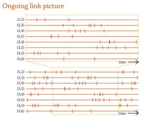
an emphasis on dynamical aspects. We find a distribution of response times (times between
consecutive contacts of different direction between two actors) that has a power law shape over a
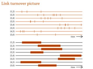
large range. We also argue that the distribution of relationship duration (the time between the
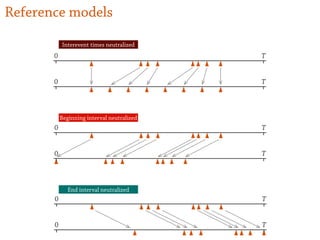
first and last contacts between actors) is exponentially decaying. Methods to reanalyze the data
to compensate for the finite sampling time are proposed. We find that the degree distribution
for networks of ongoing contacts fits better to a power law than the degree distribution of
the network of accumulated contacts do. We see that the clustering and assortative mixing
coefficients are of the same order for networks of ongoing and accumulated contacts, and that
the structural fluctuations of the former are rather large.
Introduction. – The recent development in database technology has allowed researchers
to extract very large data sets of human interaction sequences. These large data sets are
suitable to the methods and modeling techniques of statistical physics, and thus, the last years
have witnessed the appearance of an interdisciplinary field between physics and sociology [1–3].
More specifically, these studies have focused on network structure —in what ways the networks](https://image.slidesharecdn.com/tnhi-150512031650-lva1-app6891/85/Temporal-Networks-of-Human-Interaction-44-320.jpg)


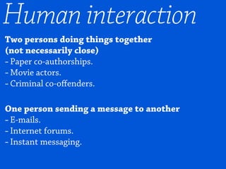
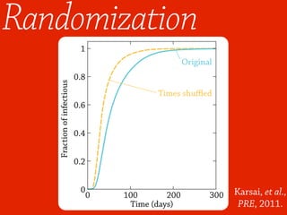
![SIR model
ds
dt
= –βsi—
di
dt
= βsi – νi—
= νi
dr
dt
—
S I I I
I R
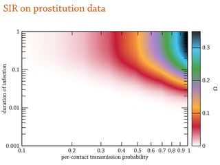
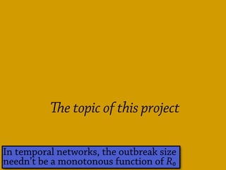
Ω = r(∞) = 1 – exp[–R₀ Ω]
where R₀ = β/ν
Ω > 0 if and only if R₀ > 1
e epidemic threshold](https://image.slidesharecdn.com/tnhi-150512031650-lva1-app6891/85/Temporal-Networks-of-Human-Interaction-64-320.jpg)


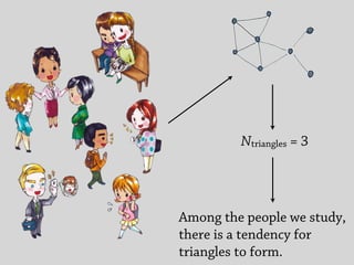
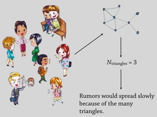
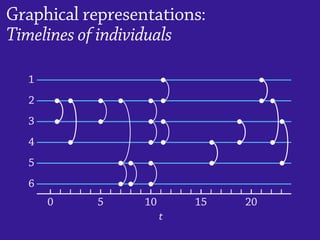
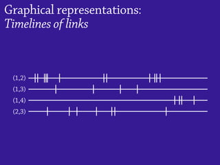
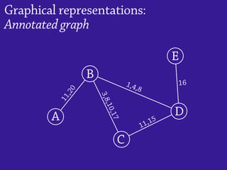
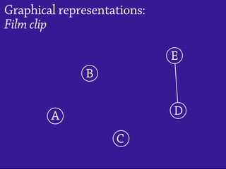
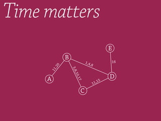
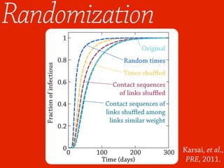
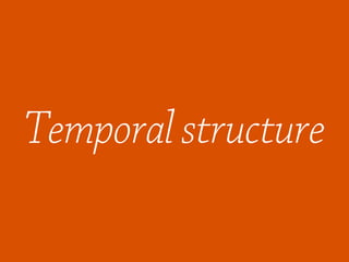
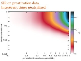
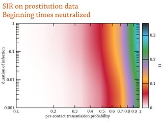
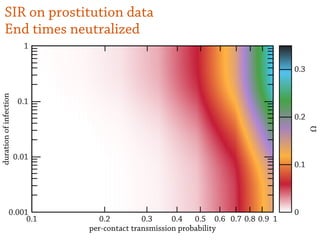
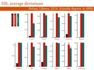
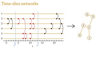
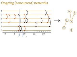
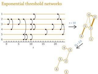
Temporal networks provide a framework for modeling systems of interactions that occur between nodes over time. These networks capture both the topological structure of connections as well as the timing of interactions. Three key aspects of temporal networks discussed in the document are: 1) Temporal networks can be represented using contact sequences that capture when interactions occur between nodes, unlike static networks which only represent connections. 2) The temporal structure of interactions, such as patterns in the timing of contacts, can impact dynamical processes unfolding on the network like information or disease spreading. 3) Randomizing the timing of contacts in empirical temporal network data can alter dynamical processes, highlighting the importance of temporal structure beyond just topology.


![Polymer [ बहुलक ] Chemistry Notes PDF - Irfanullah Mehar - JJ Sir Chemistry.pdf](https://cdn.slidesharecdn.com/ss_thumbnails/polymerchemistrynotespdf-irfanullahmehar-jjsirchemistry-260210172118-3f9b37f7-thumbnail.jpg?width=640&height=640&fit=bounds)