Downloaded 11 times
![Overfitting
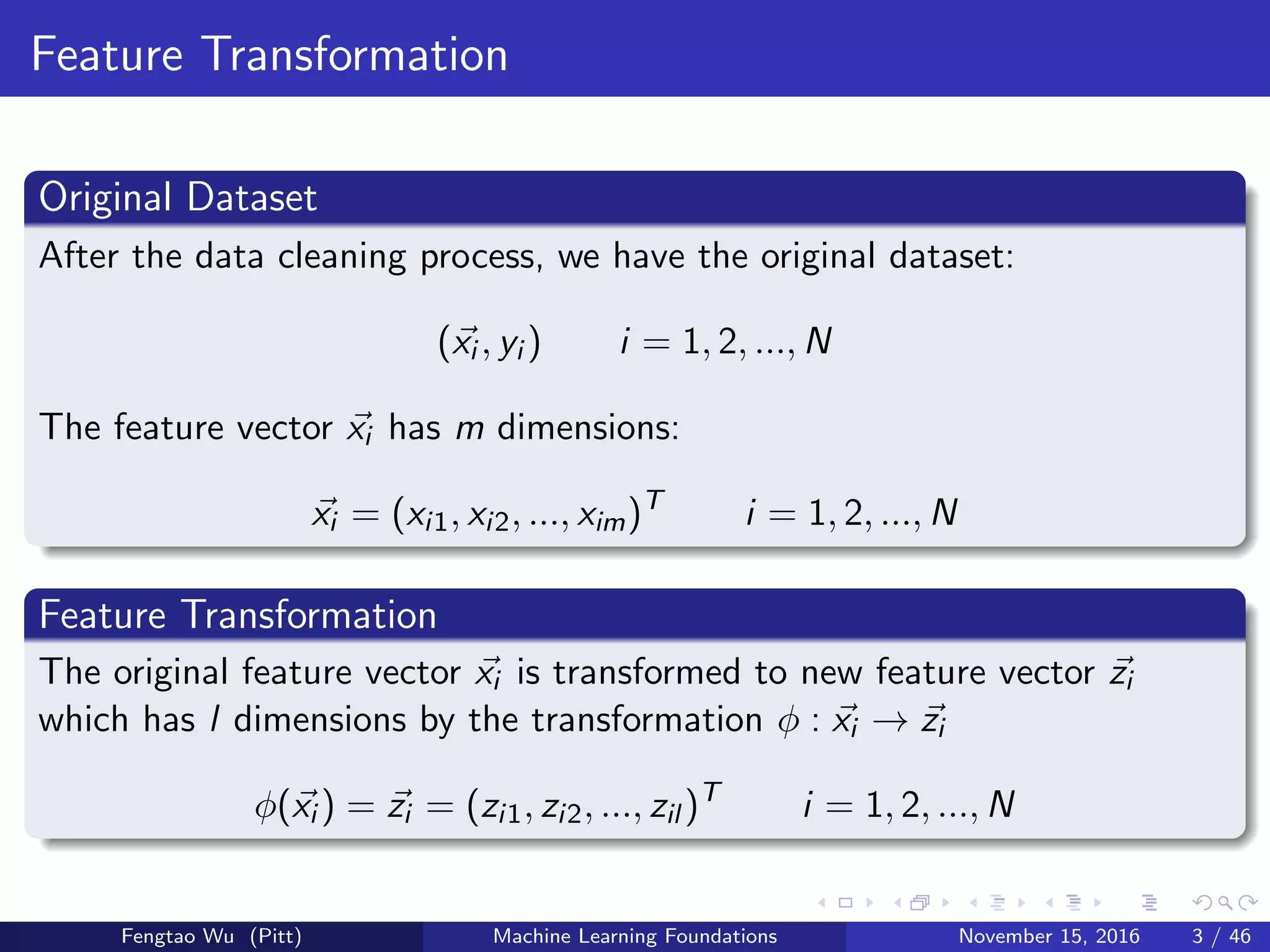
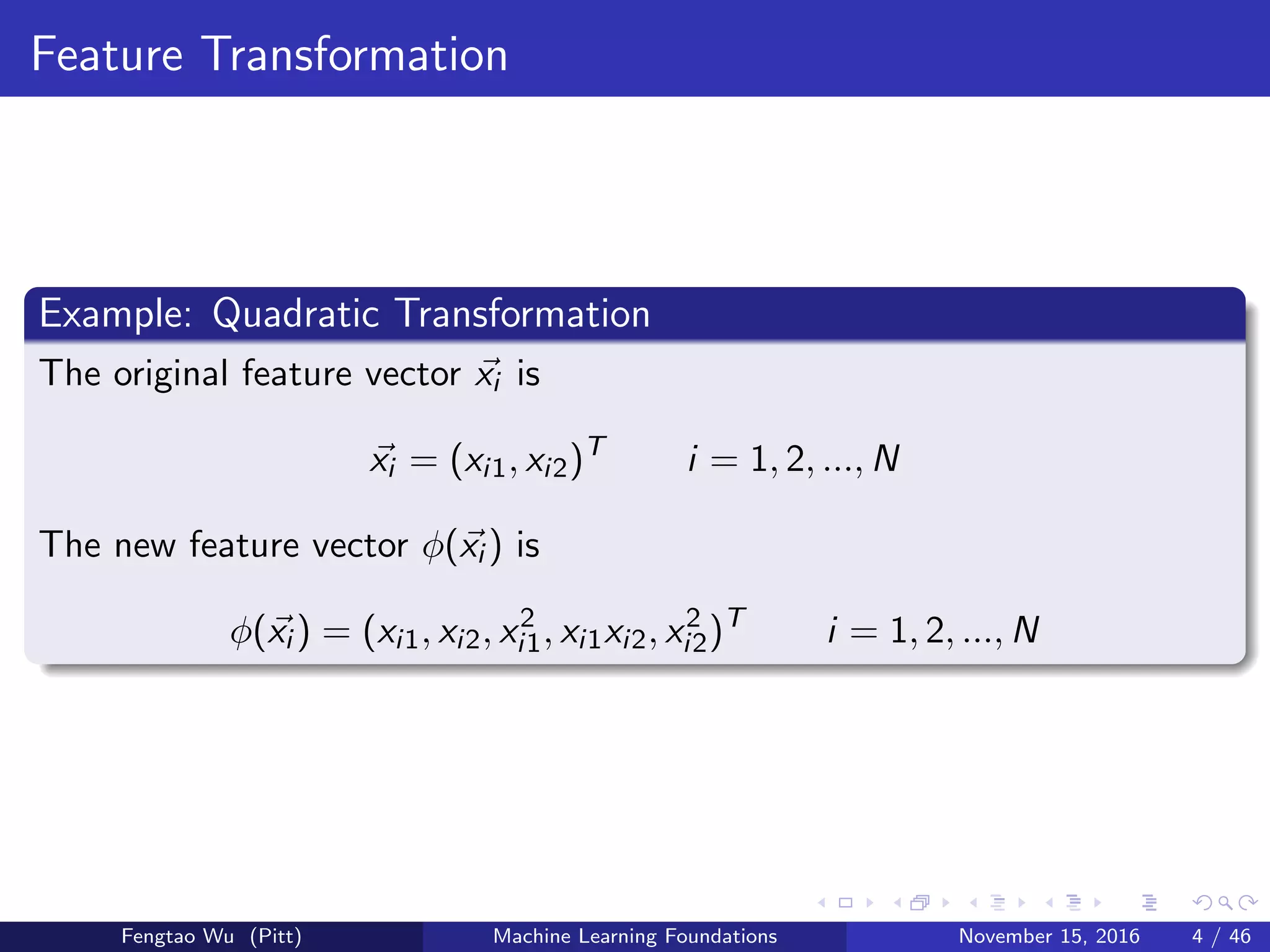
The feature transformation may cause the overfitting problem:
φ(xi ) = (xi , x2
i , x3
i , ..., x10
i )T
i = 1, 2, ..., N
Figure: Polynomial transformation cause overfitting problem, from [Wikipedia].
Fengtao Wu (Pitt) Machine Learning Foundations November 15, 2016 5 / 46](https://image.slidesharecdn.com/a56bde66-f392-4c31-88bb-47293941ecb1-170102203834/75/Linear-Machine-Learning-Models-with-L2-Regularization-and-Kernel-Tricks-5-2048.jpg)
![Geometric Interpretation of L2-Regularization
L2-Regularization
The optimal w∗ satisfies:
− Ein(ω∗) ω∗
i.e.
Ein(ω∗) +
2λ
N
ω∗ = 0
i.e.
min
ω
Ein(ω) +
λ
N
ωT
ω
Geometric Interpretation
Figure: Interpretation of
L2-regularization, from [Lin].
Fengtao Wu (Pitt) Machine Learning Foundations November 15, 2016 10 / 46](https://image.slidesharecdn.com/a56bde66-f392-4c31-88bb-47293941ecb1-170102203834/75/Linear-Machine-Learning-Models-with-L2-Regularization-and-Kernel-Tricks-10-2048.jpg)
![Quadratic Programming [Burke]
QP Standard Form
The standard form of quadratic programming Q is
min
x
1
2
xT
Qx + cT
x
s.t. Ax ≥ b
where A ∈ IRm×n
and b ∈ IRm
, and the matrix Q is symmetric. In the QP
standard form, the number of unknown variables is n, and the number of
constraints is m.
Fengtao Wu (Pitt) Machine Learning Foundations November 15, 2016 14 / 46](https://image.slidesharecdn.com/a56bde66-f392-4c31-88bb-47293941ecb1-170102203834/75/Linear-Machine-Learning-Models-with-L2-Regularization-and-Kernel-Tricks-14-2048.jpg)
![QP Solver [Hoppe]
Direct Solution
Symmetric Indefinite Factorization
Range-Space Approach
Null-Space Approach
Iterative Solution
Krylov Methods
Transforming Range-Space Iterations
Transforming Null-Space Iterations
Active Set Strategies for Convex QP Problems
Primal Active Set Strategies
Primal-dual Active Set Strategies
Fengtao Wu (Pitt) Machine Learning Foundations November 15, 2016 17 / 46](https://image.slidesharecdn.com/a56bde66-f392-4c31-88bb-47293941ecb1-170102203834/75/Linear-Machine-Learning-Models-with-L2-Regularization-and-Kernel-Tricks-17-2048.jpg)
![Hard-Margin SVM Primal Lagrangian Function
Hard-Margin SVM Primal Lagrangian Function
The Lagrangian function is
L(b, ω, α) =
1
2
ωT
ω +
N
n=1
αn[1 − yn(ωT
zn + b)]
where α ≥ 0 and α is called Lagrangian Multipliers.
Hard-Margin SVM Primal Equivalent
Hard-Margin SVM Primal ⇐⇒ min
b,ω
(max
α
L(b, ω, α))
Fengtao Wu (Pitt) Machine Learning Foundations November 15, 2016 19 / 46](https://image.slidesharecdn.com/a56bde66-f392-4c31-88bb-47293941ecb1-170102203834/75/Linear-Machine-Learning-Models-with-L2-Regularization-and-Kernel-Tricks-19-2048.jpg)
![Probabilistic SVM [Platt, 1999]
Platt’s Model of Probabilistic SVM for Soft-Binary Classification
The probabilistic SVM model is
Θ(x) = 1/(1 + exp(−x))
h(x) = Θ(A(ωSVM
T
Φ(x) + bSVM) + B)
P(y|z) =
h(z) if y = +1
1 − h(z) if y = −1
A functions as scaling: often A > 0 if ωSVM is reasonably good
B functions as shifting: often B ≈ 0 if bSVM is reasonably good
Two-level learning: logistic regression on SVM-transformed data
Fengtao Wu (Pitt) Machine Learning Foundations November 15, 2016 26 / 46](https://image.slidesharecdn.com/a56bde66-f392-4c31-88bb-47293941ecb1-170102203834/75/Linear-Machine-Learning-Models-with-L2-Regularization-and-Kernel-Tricks-26-2048.jpg)
![Gaussian Kernel
Gaussian Kernel
K(x1, x2) = exp(−γ x1 − x2
2
)
e.g.
K(x1, x2) = exp(−(x1 − x2)2
)
= exp(−x2
1 ) exp(−x2
2 ) exp(2x1x2)
= exp(−x2
1 ) exp(−x2
2 )(
∞
i=0
(2x1x2)i
i!
)
=
∞
i=0
[
2i
i!
exp(−x2
1 )xi
1][
2i
i!
exp(−x2
2 )xi
2]
Φ(x) = exp(−x2
)(1,
2
1!
x,
22
2!
x2
, · · · )
Fengtao Wu (Pitt) Machine Learning Foundations November 15, 2016 29 / 46](https://image.slidesharecdn.com/a56bde66-f392-4c31-88bb-47293941ecb1-170102203834/75/Linear-Machine-Learning-Models-with-L2-Regularization-and-Kernel-Tricks-29-2048.jpg)
![Mercer’s Condition [Wikipedia]
Mercer’s Condition
The function KΦ : X × X → IR, KΦ(xi , xj ) = Φ(xi )T Φ(xj ) is
symmetric
Define
Z =
Φ(x1)T
...
Φ(xN)T
K = ZZT
The matrix K is positive semi-definite.
Fengtao Wu (Pitt) Machine Learning Foundations November 15, 2016 30 / 46](https://image.slidesharecdn.com/a56bde66-f392-4c31-88bb-47293941ecb1-170102203834/75/Linear-Machine-Learning-Models-with-L2-Regularization-and-Kernel-Tricks-30-2048.jpg)
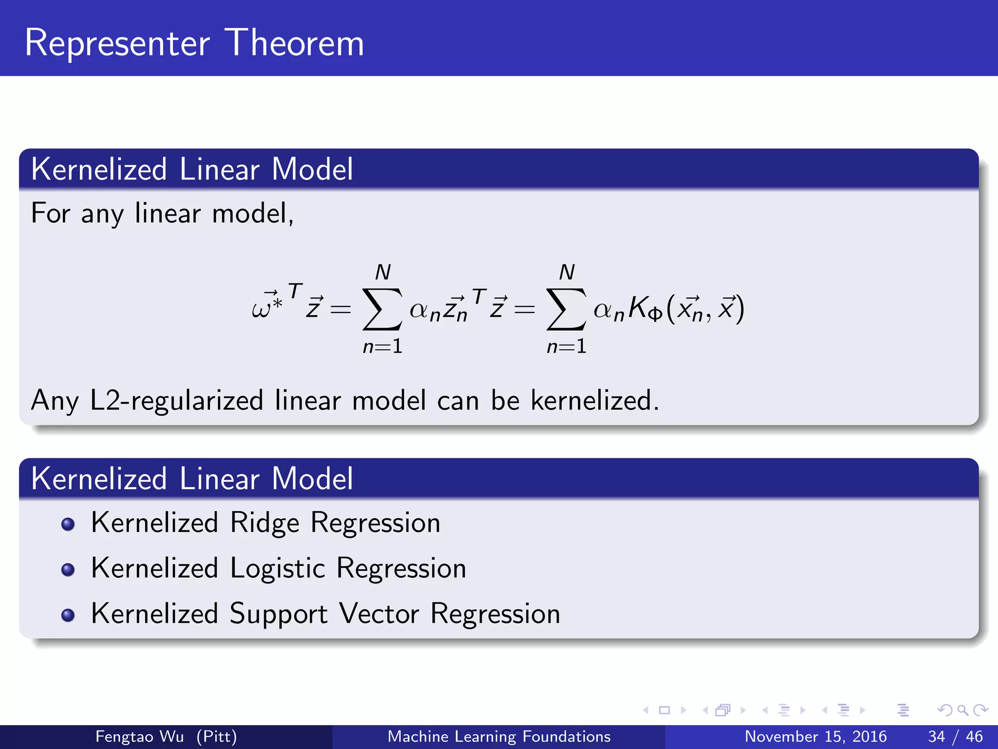
![Representer Theorem
[Schlkopf, Herbrich and Smola, 2001]
Theorem (Representer Theorem)
For any L2-regularized linear model,
min
ω
λ
N
ωT
ω +
1
N
N
n=1
Ein(yn, ωT
zn)
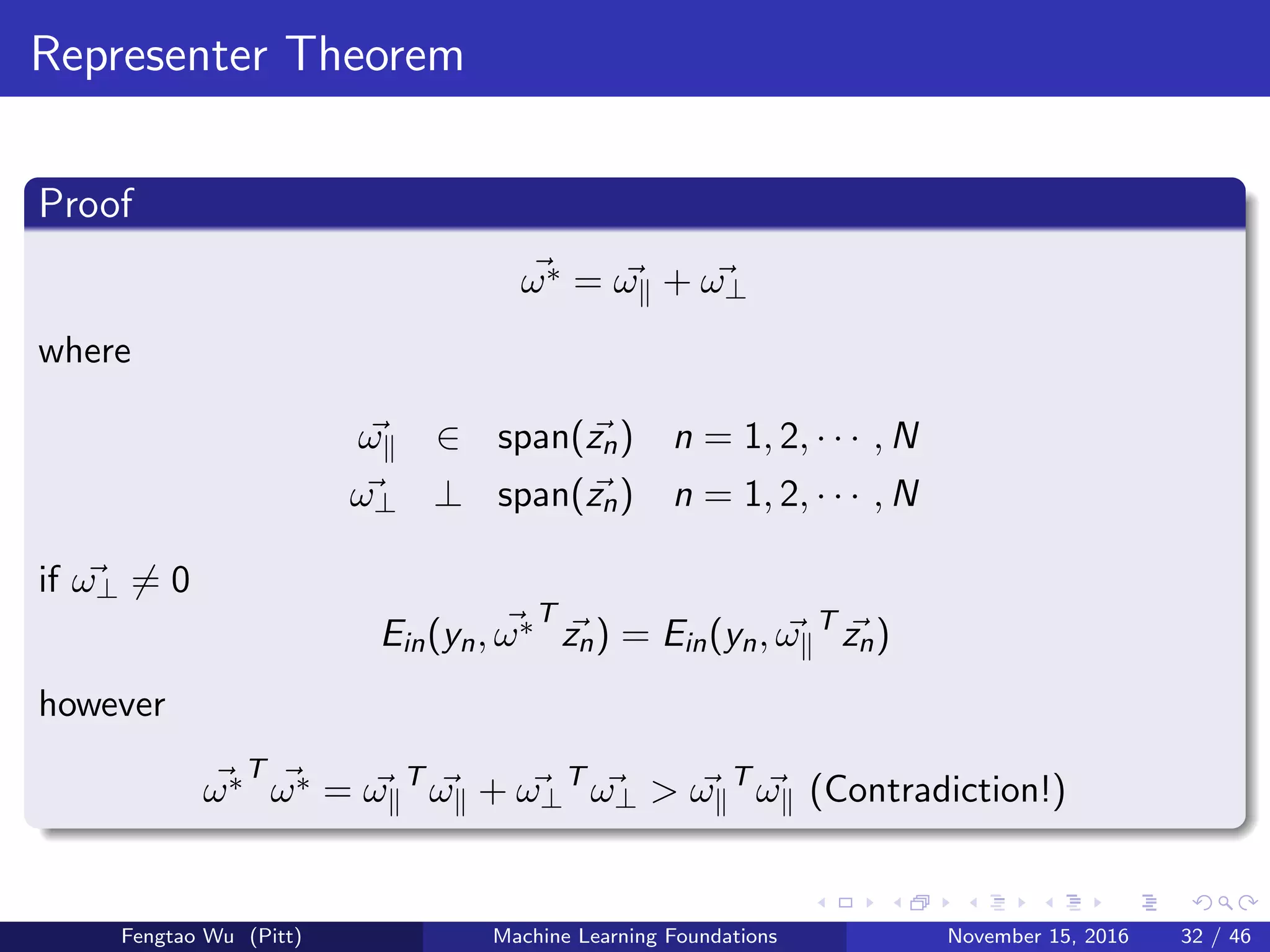
The optimal ω∗ satisfies:
ω∗ =
N
n=1
αnzn = ZT
α
Fengtao Wu (Pitt) Machine Learning Foundations November 15, 2016 31 / 46](https://image.slidesharecdn.com/a56bde66-f392-4c31-88bb-47293941ecb1-170102203834/75/Linear-Machine-Learning-Models-with-L2-Regularization-and-Kernel-Tricks-31-2048.jpg)
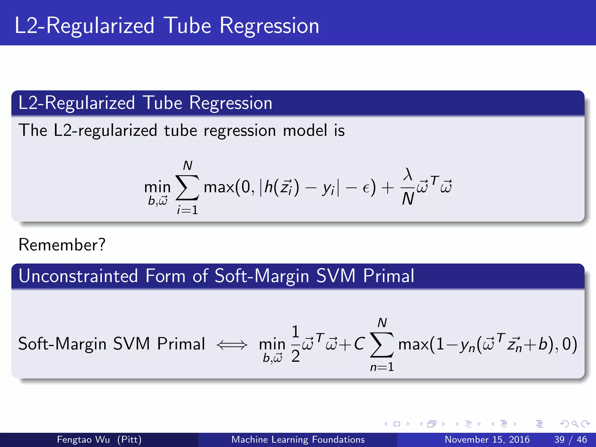
![Tube Regression
Tube Regression
The tube regression model is
h(z) = ωT
z + b
The error function of the model is
Ein(h) =
N
i=1
max(0, |h(zi )−yi |− )
Tube Regression
Figure: Interpretation of tube
regularization, from [ResearchGate].
Fengtao Wu (Pitt) Machine Learning Foundations November 15, 2016 38 / 46](https://image.slidesharecdn.com/a56bde66-f392-4c31-88bb-47293941ecb1-170102203834/75/Linear-Machine-Learning-Models-with-L2-Regularization-and-Kernel-Tricks-38-2048.jpg)
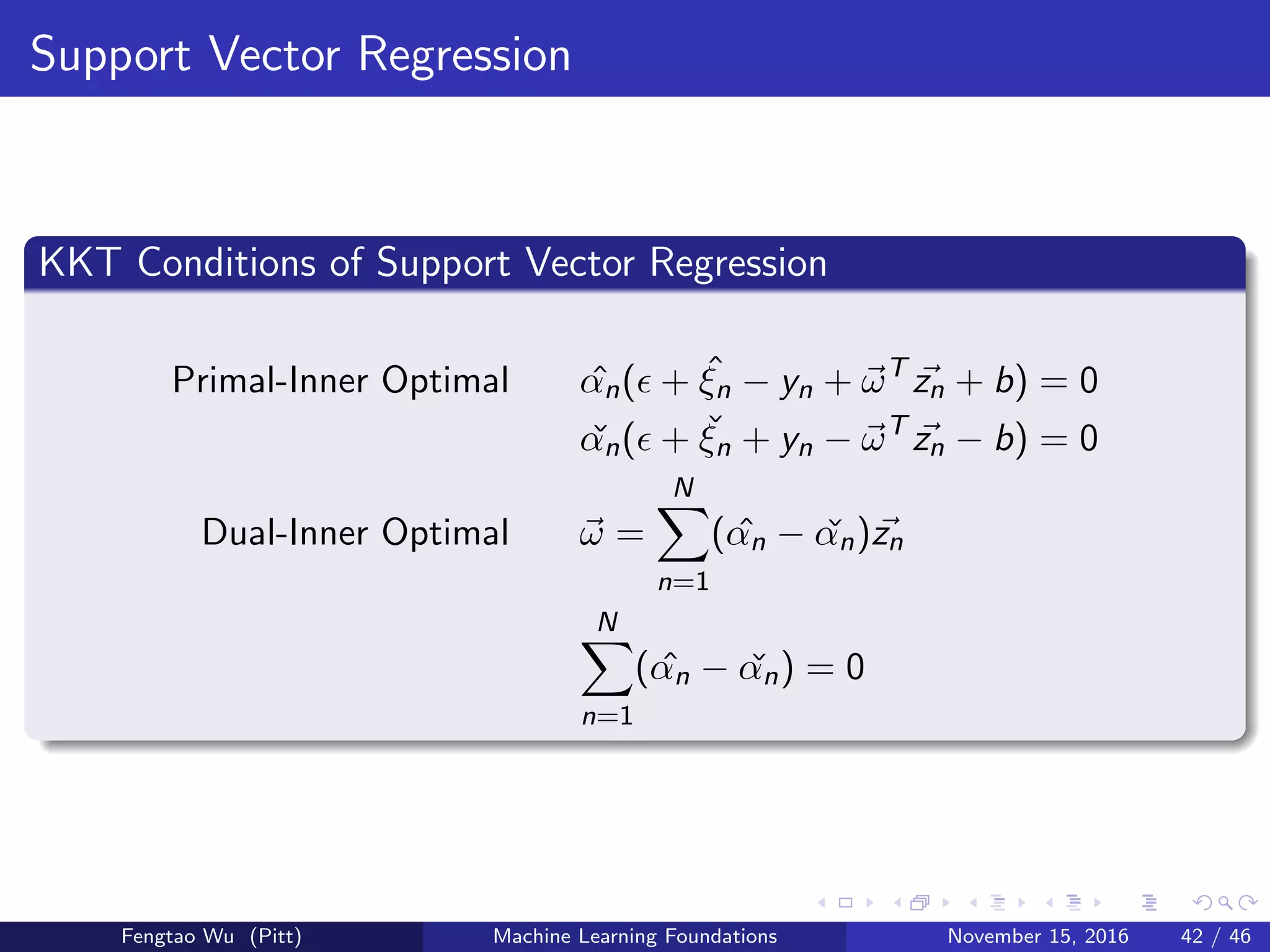
![Support Vector Regression [Welling, 2004]
SVR Primal: solve l + 1 + 2N variables under 4N constraints
Support Vector Regression
Primal
min
b,ω,ξ
1
2
ωT
ω + C
N
n=1
ξn
s.t. |ωT
zn + b − yn| ≤ + ξn
ξn ≥ 0
n = 1, 2, ..., N
Support Vector Regression Primal
Refinement
min
b,ω,ˆξ,ˇξ
1
2
ωT
ω + C
N
n=1
( ˆξn + ˇξn)
s.t. −b − ωT
zn + ˆξn ≥ − − yn
b + ωT
zn + ˇξn ≥ − + yn
ˆξn ≥ 0
ˇξn ≥ 0
n = 1, 2, ..., N
Fengtao Wu (Pitt) Machine Learning Foundations November 15, 2016 40 / 46](https://image.slidesharecdn.com/a56bde66-f392-4c31-88bb-47293941ecb1-170102203834/75/Linear-Machine-Learning-Models-with-L2-Regularization-and-Kernel-Tricks-40-2048.jpg)
![Support Vector Regression
SVR Dual: solve 2N variables under 4N + 1 constraints
Kernelized Support Vector Regression Dual
min
b,ω,ξ
1
2
N
n=1
N
m=1
( ˆαn − ˇαn)( ˆαm − ˇαm)kn,m
+
N
n=1
[( − yn) ˆαn + ( + yn) ˇαn]
s.t.
N
n=1
( ˆαn − ˇαn) = 0
0 ≤ ˆαn ≤ C
0 ≤ ˇαn ≤ C
n = 1, 2, ..., N
Fengtao Wu (Pitt) Machine Learning Foundations November 15, 2016 41 / 46](https://image.slidesharecdn.com/a56bde66-f392-4c31-88bb-47293941ecb1-170102203834/75/Linear-Machine-Learning-Models-with-L2-Regularization-and-Kernel-Tricks-41-2048.jpg)

The document covers linear machine learning models, specifically focusing on l2-regularization and kernel tricks. It discusses feature transformation, overfitting, linear regression, logistic regression, and the principles of quadratic programming related to support vector machines (SVMs). Key concepts such as regularization methods, duality in optimization, and popular kernel functions are also explored.
Overview of Linear Machine Learning Models focusing on L2-Regularization and Kernel Tricks.
Discusses feature transformation from original datasets, including overfitting risks related to transformations.
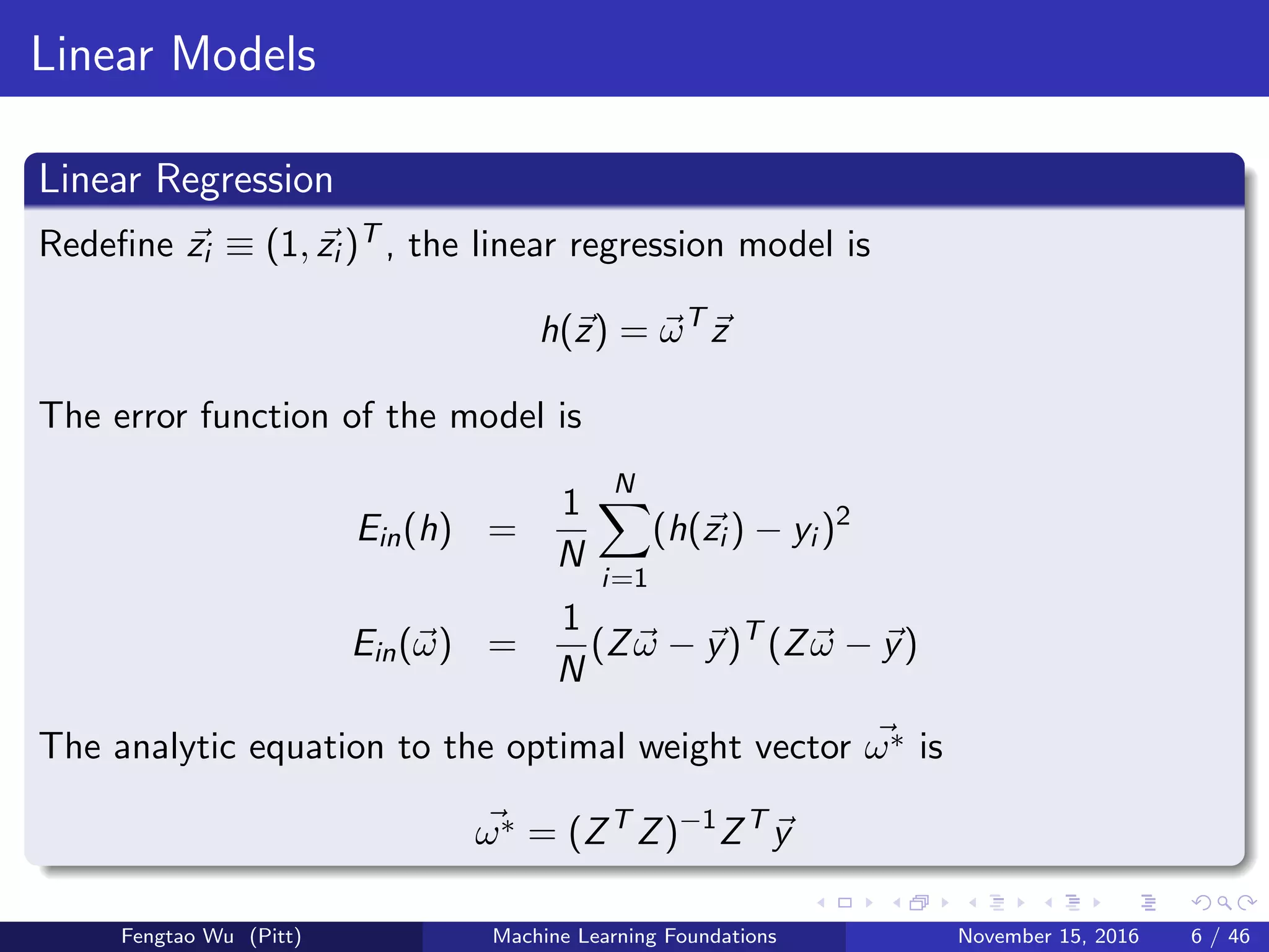
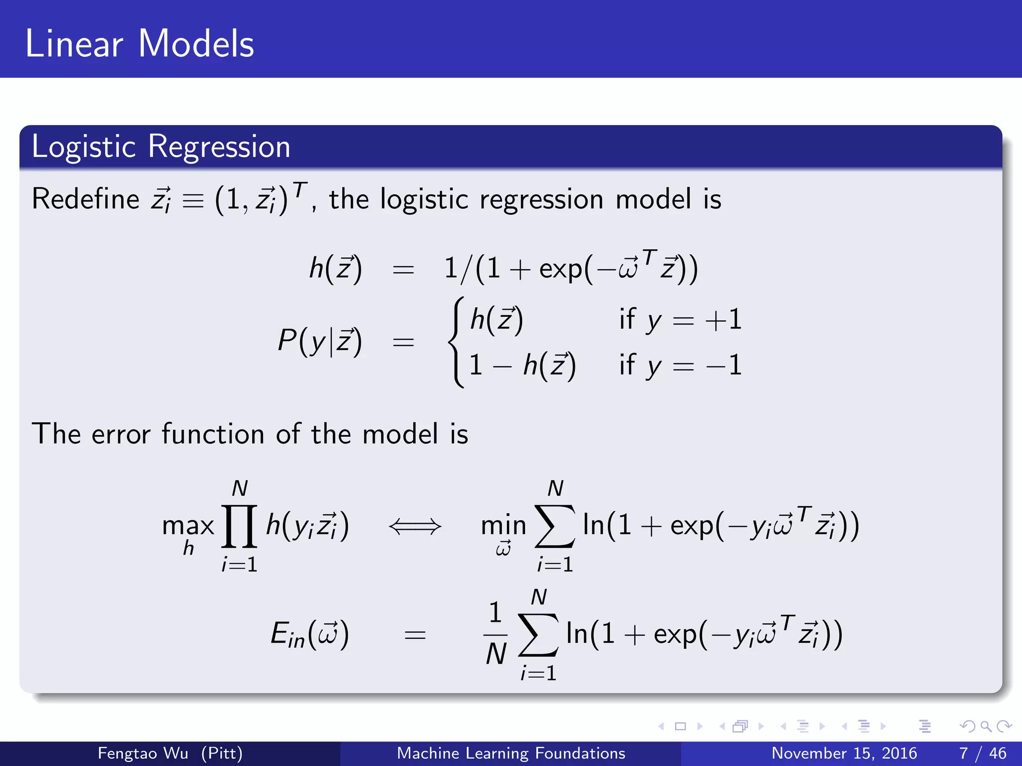
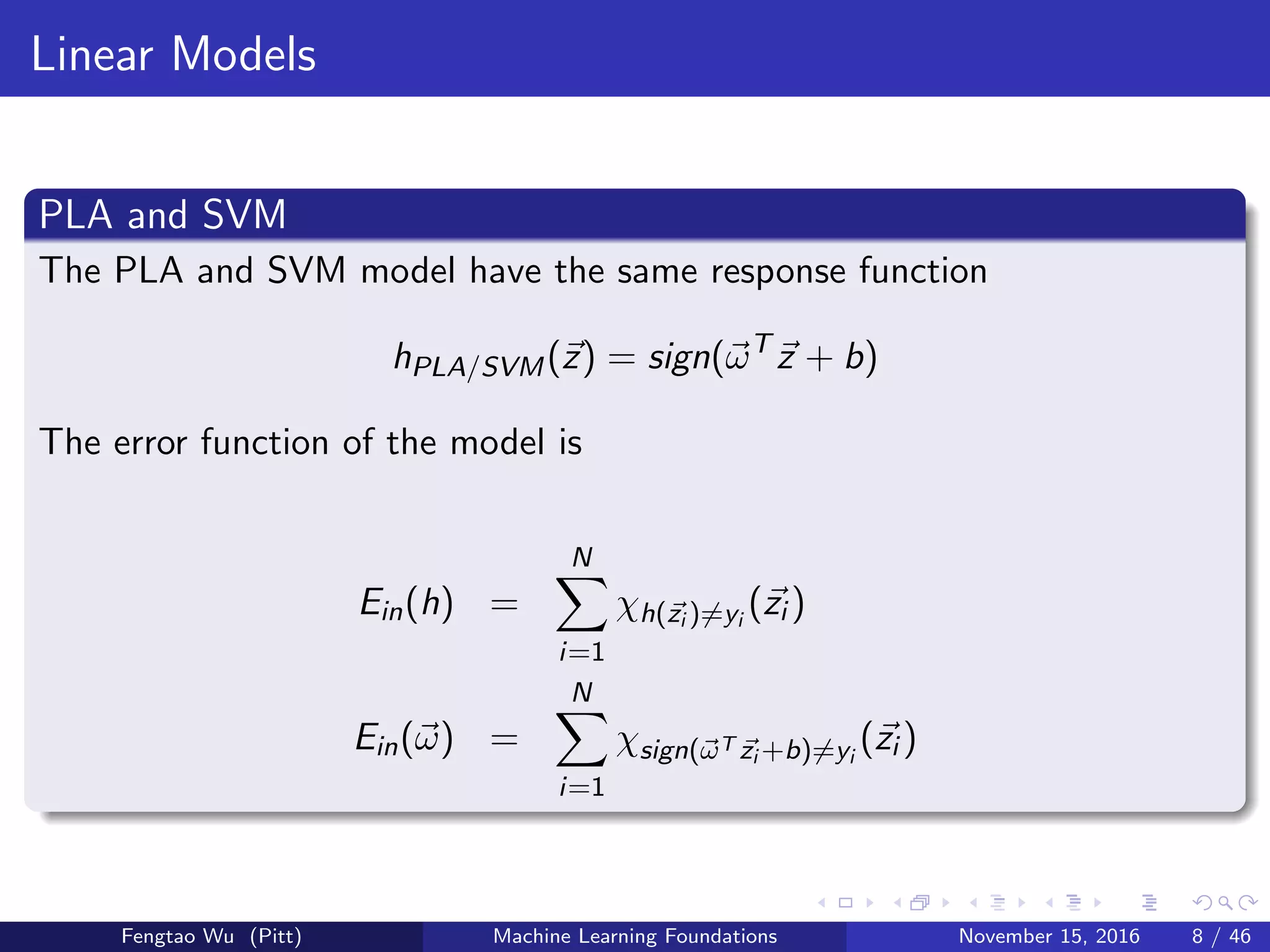
Introduces linear regression, logistic regression, and PLA/SVM models, detailing error functions and weight calculations.
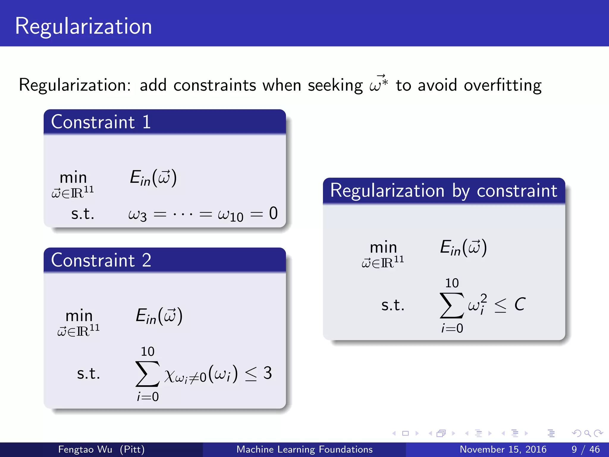
Explains regularization to avoid overfitting, focusing on L2-regularization and its geometric interpretation.
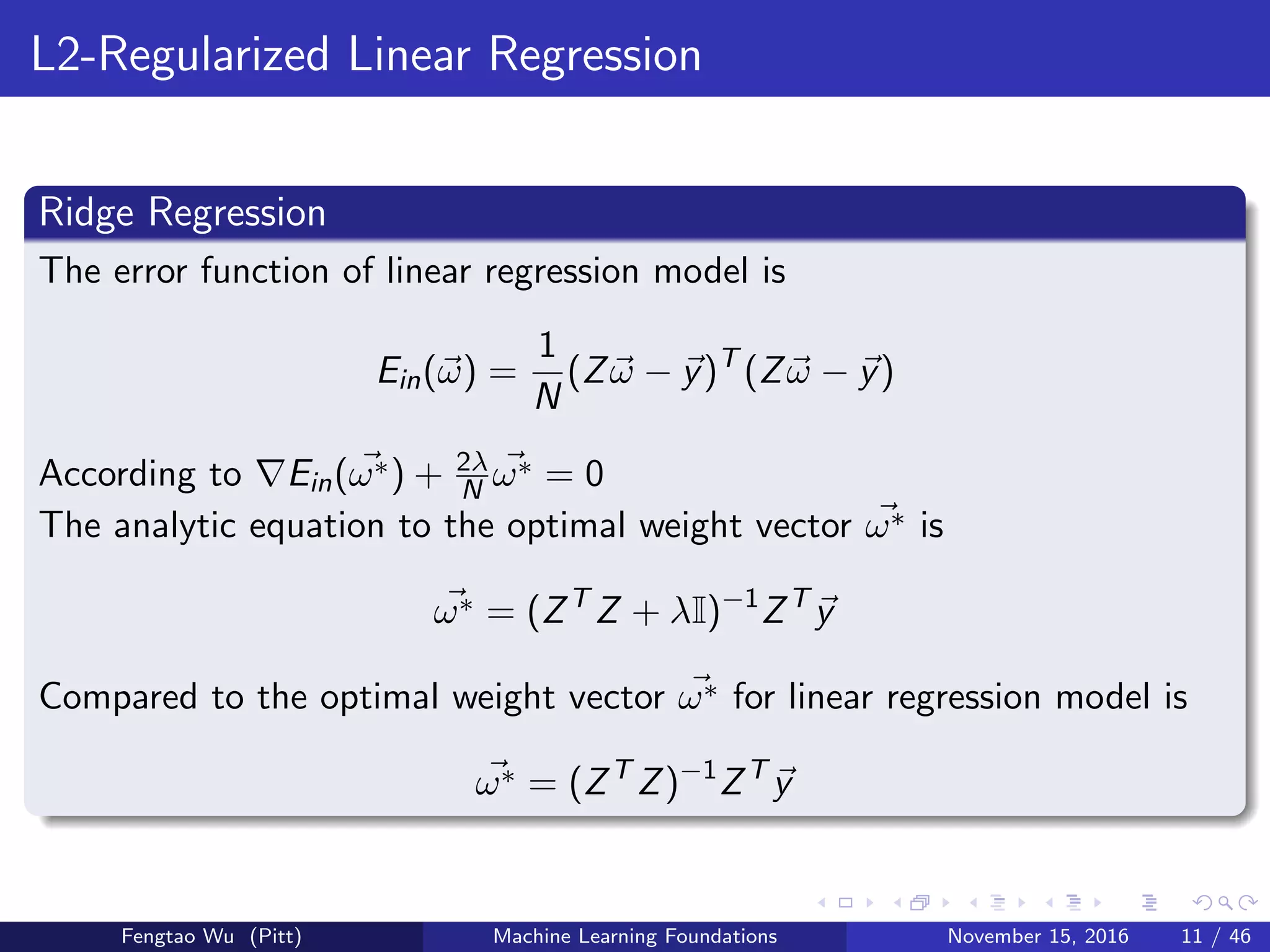
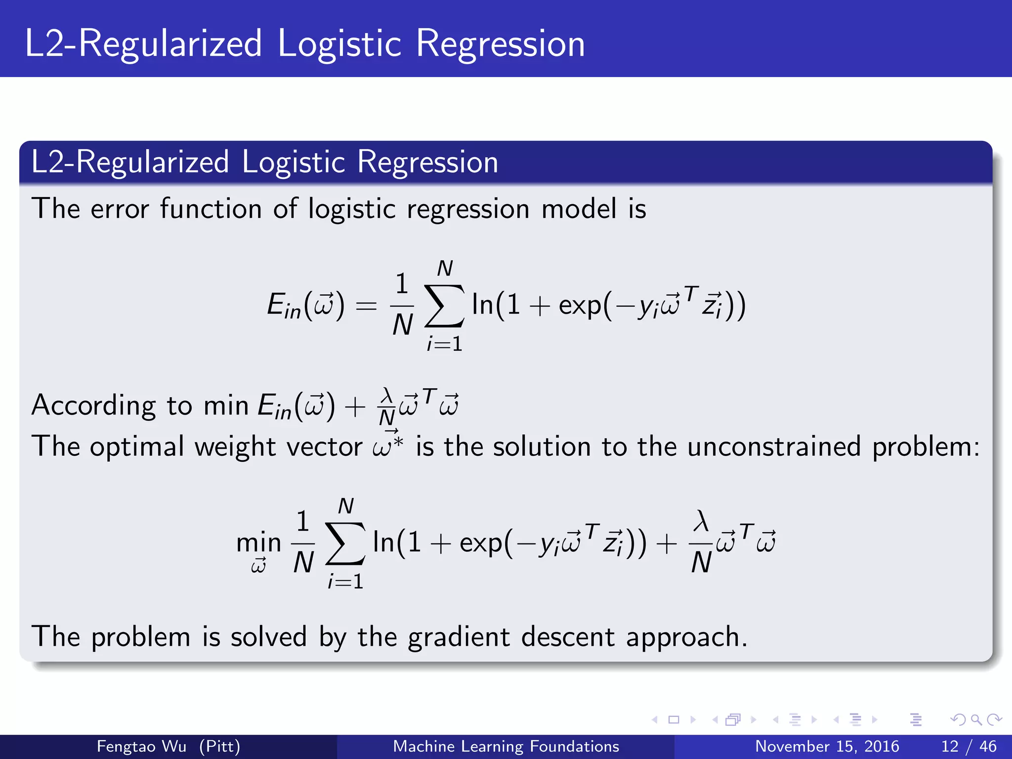
Details analytic equations for Ridge and Logistic regression under L2-regularization and concept of weight decay.
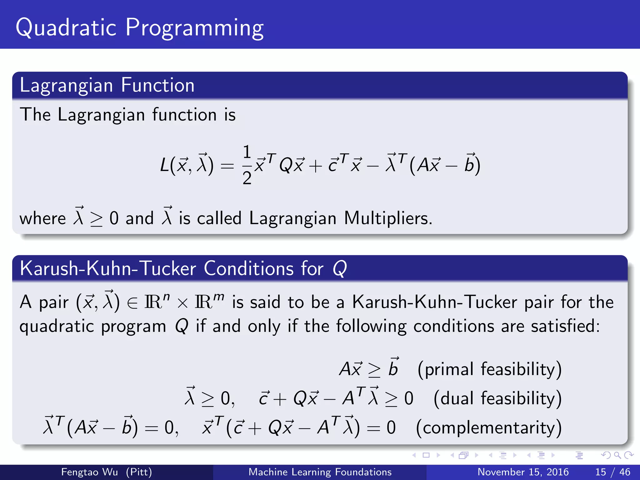
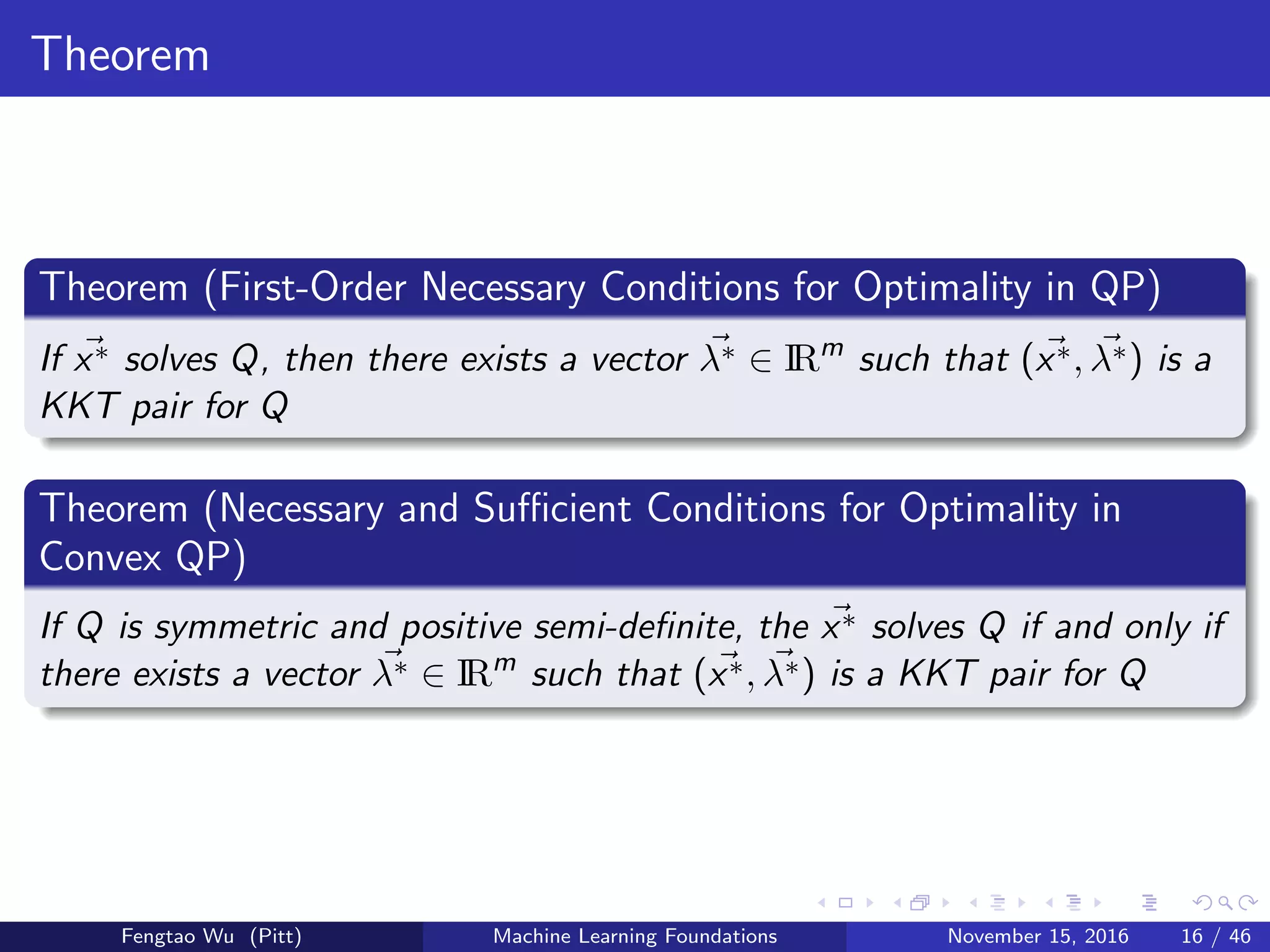
Introduces Quadratic Programming, its standard form, Lagrangian function, and necessary conditions for optimality.
Describes direct and iterative solutions for Quadratic Programming including methods for solving various QP forms.
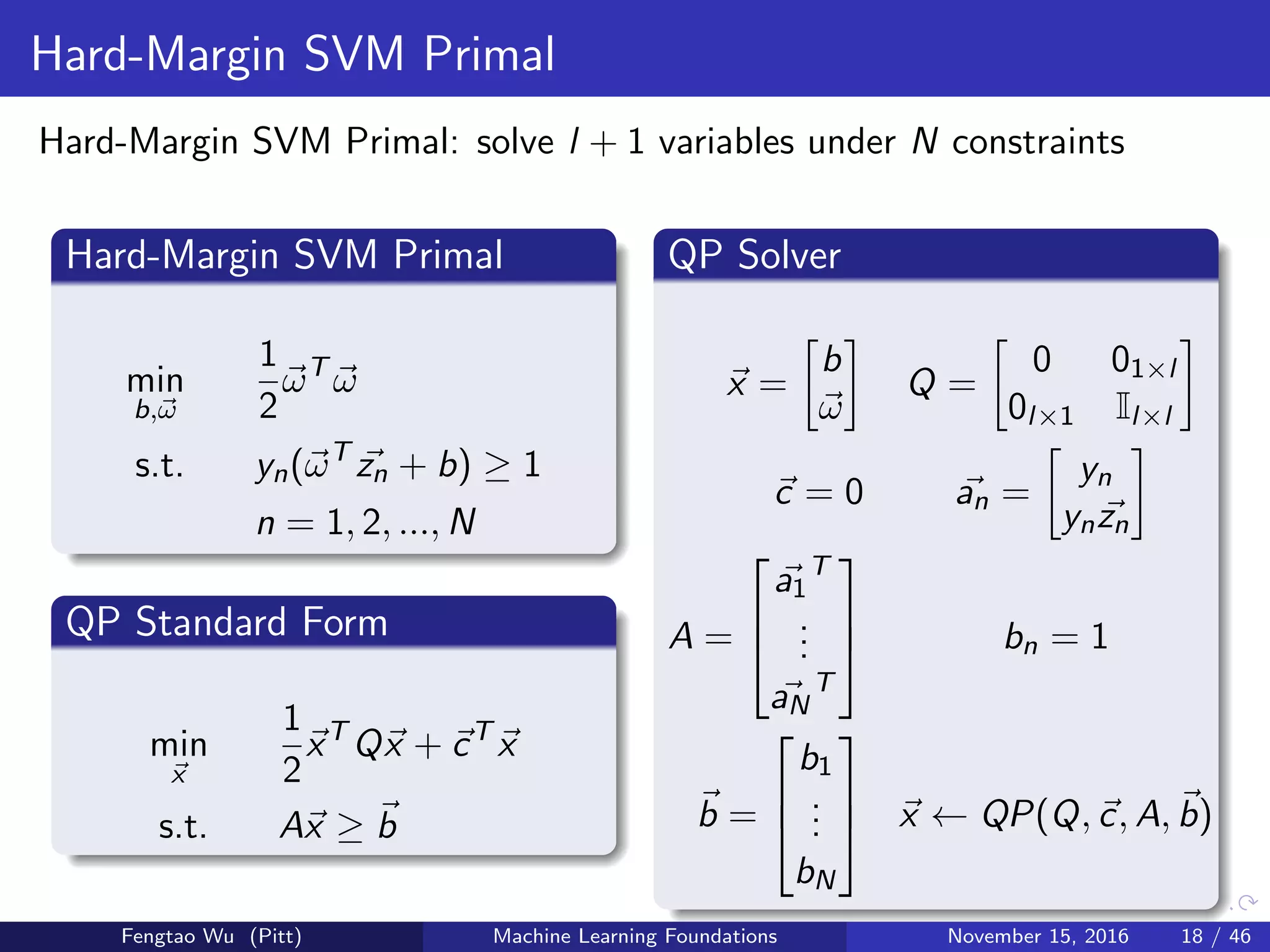
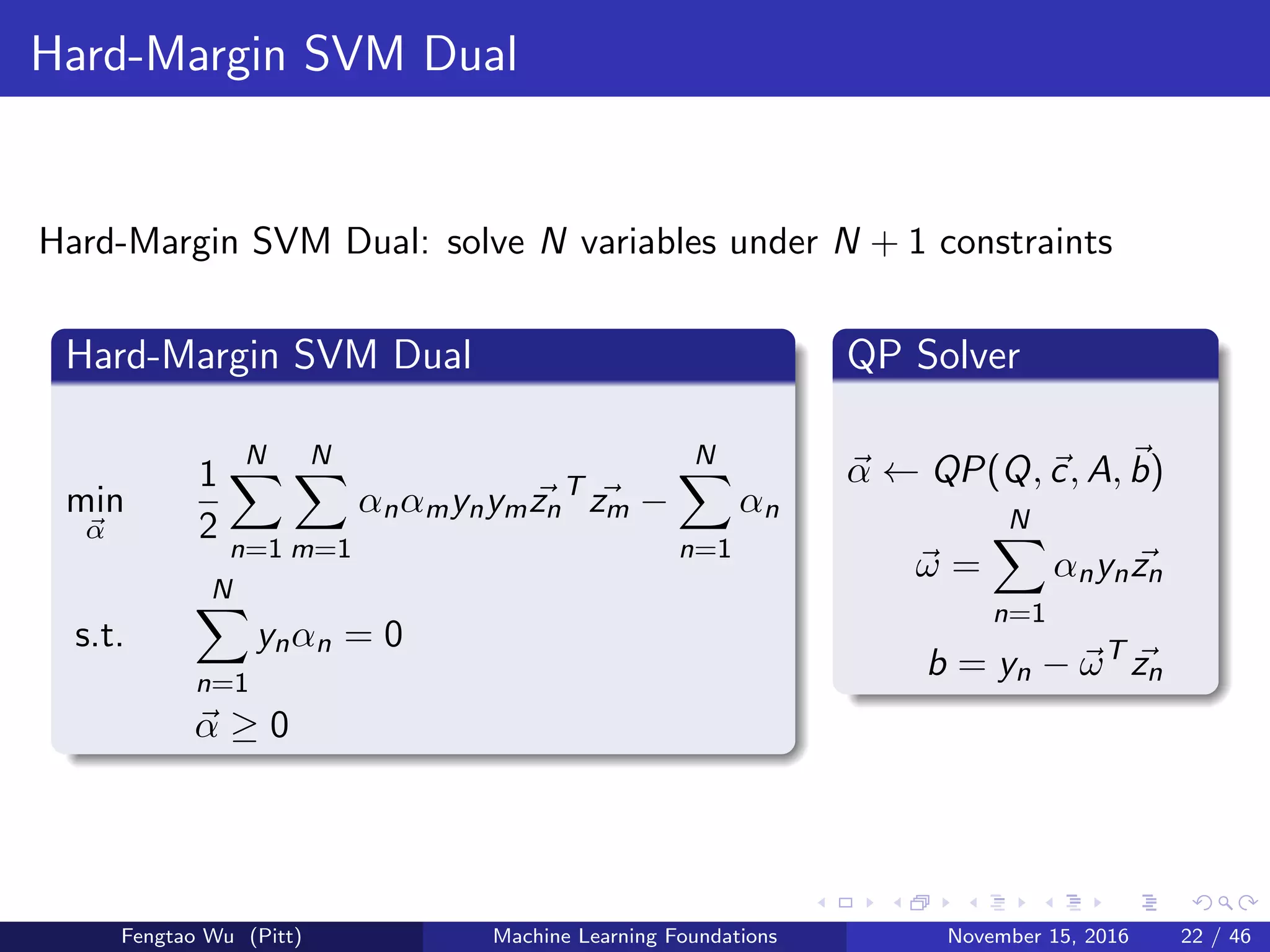
Describes the primal forms for Hard-Margin SVM including Lagrangian functions and equivalents.
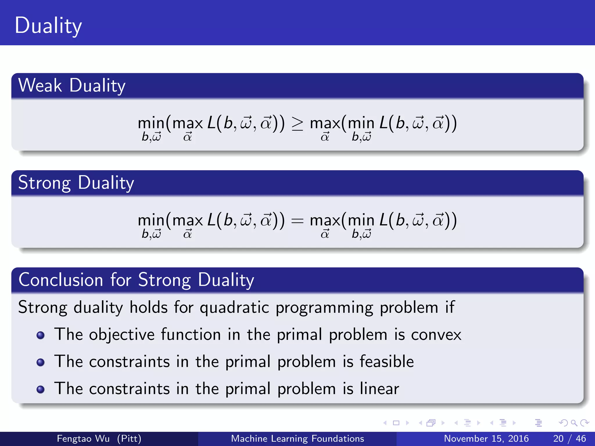
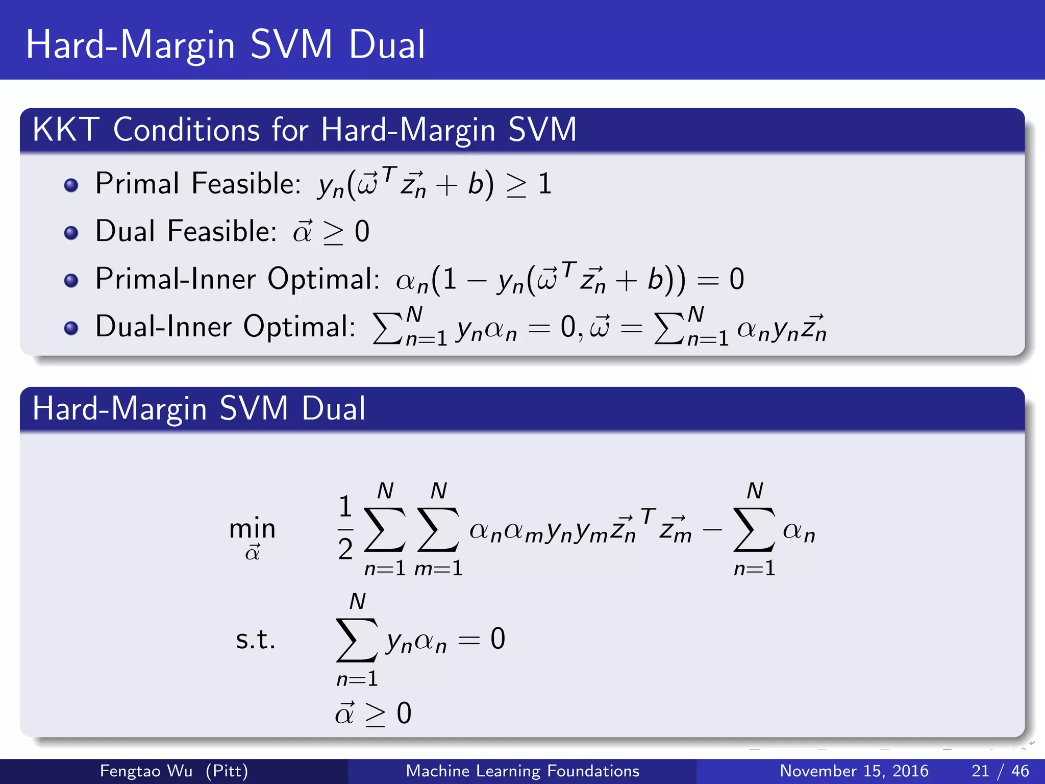
Discusses weak and strong duality principles in quadratic programming related to SVM problems.
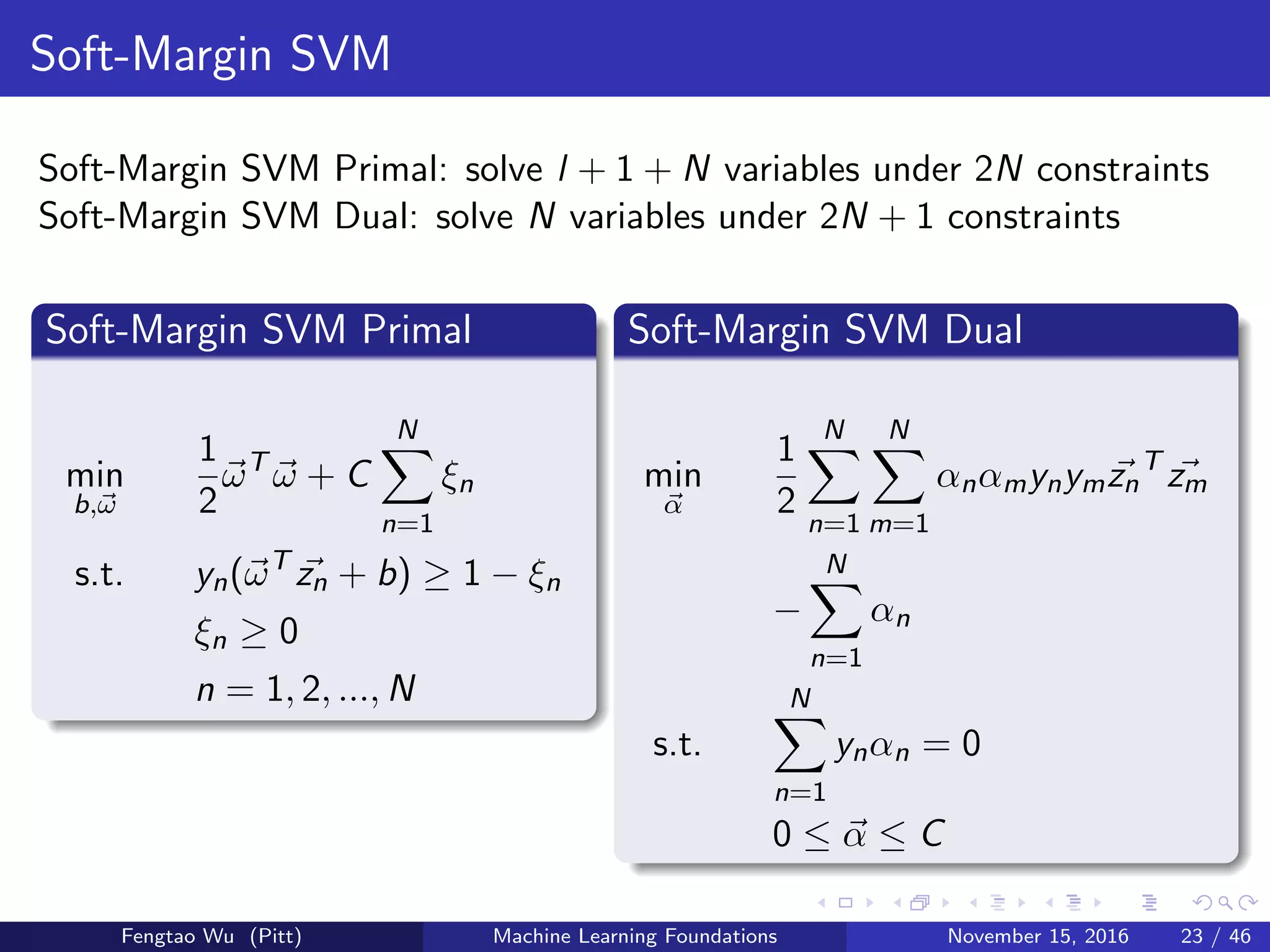
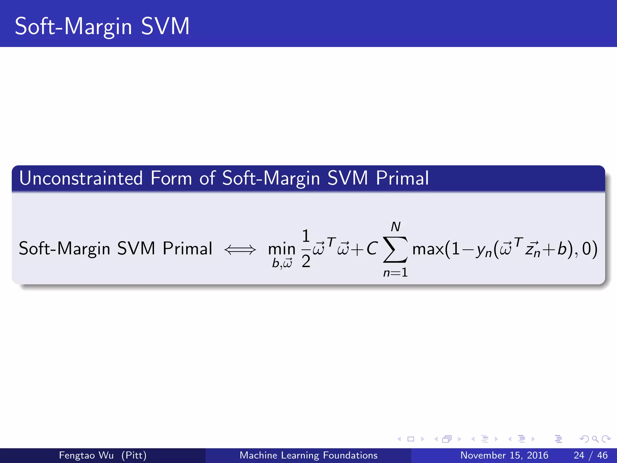
Details the primal and dual formulations of Soft-Margin SVM with constraints and performance criteria.
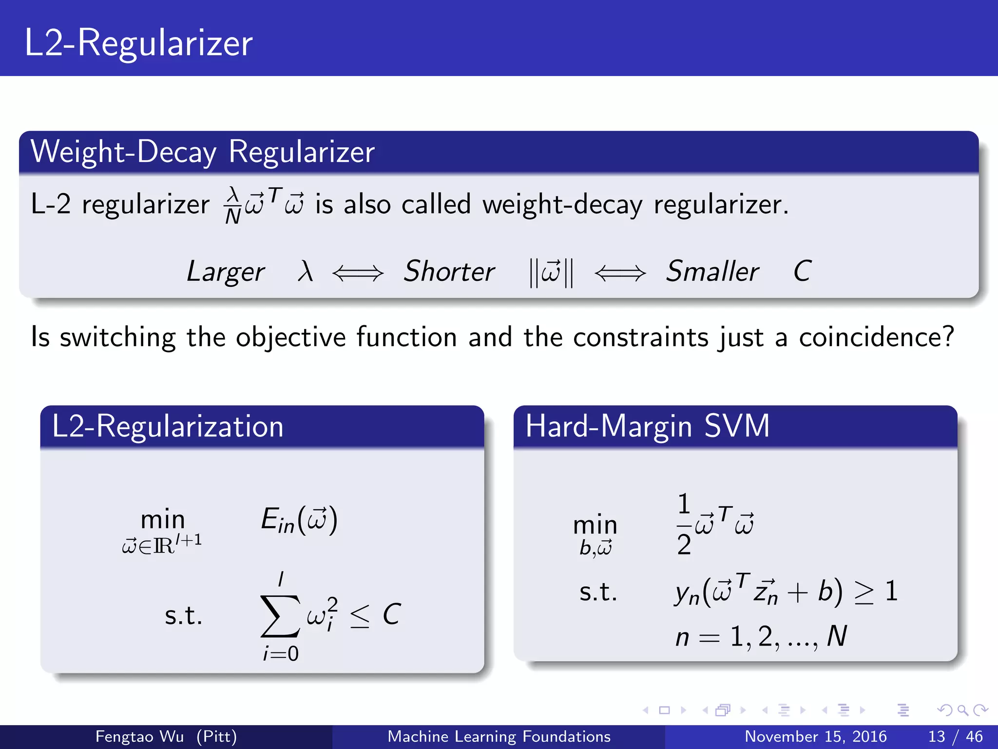
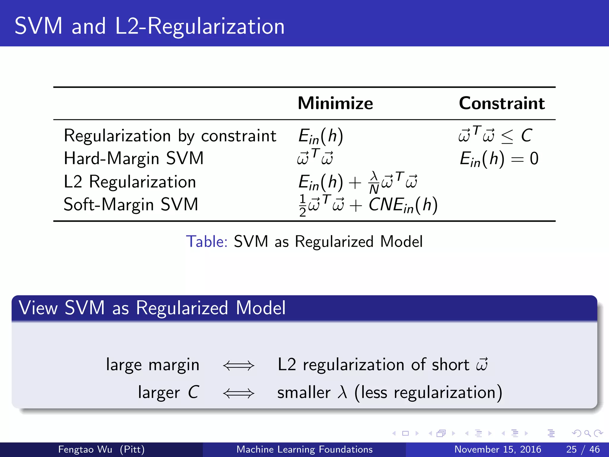
Explains the relationship between SVM optimization principles and L2-Regularization.
Introduces Platt's model of Probabilistic SVM for binary classification.
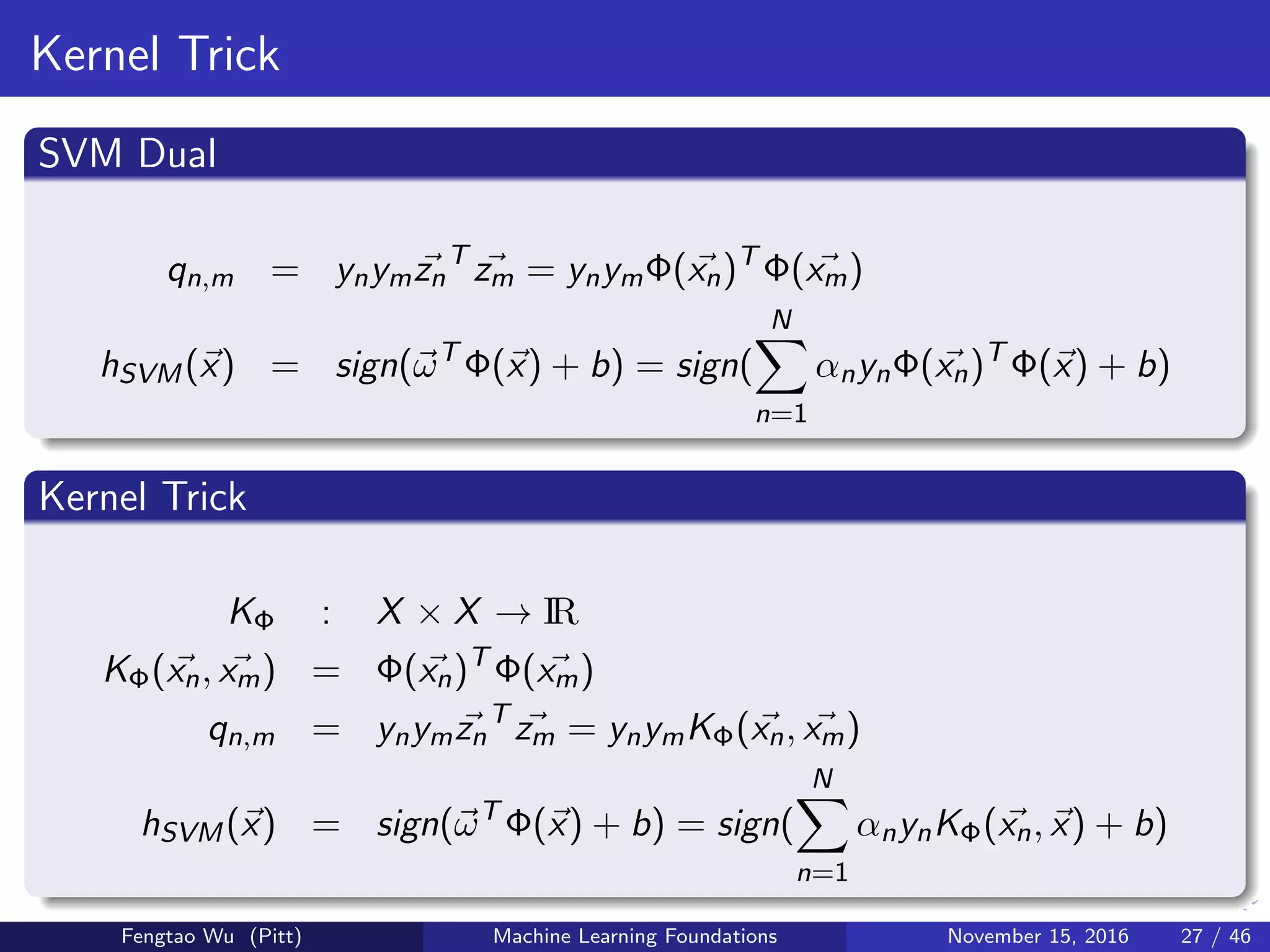
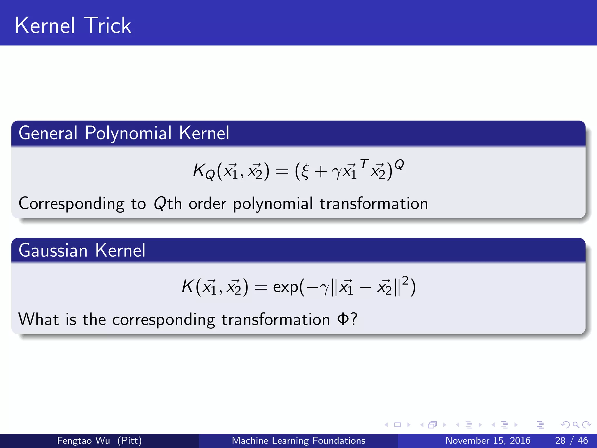
Explains the Kernel Trick, including polynomial and Gaussian kernels, facilitating complex transformations.
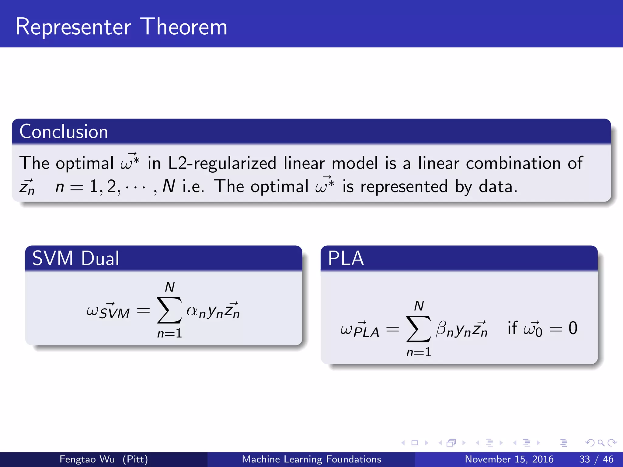
Details Mercer's Condition for symmetric functions and the Representer Theorem regarding L2-regularized models.
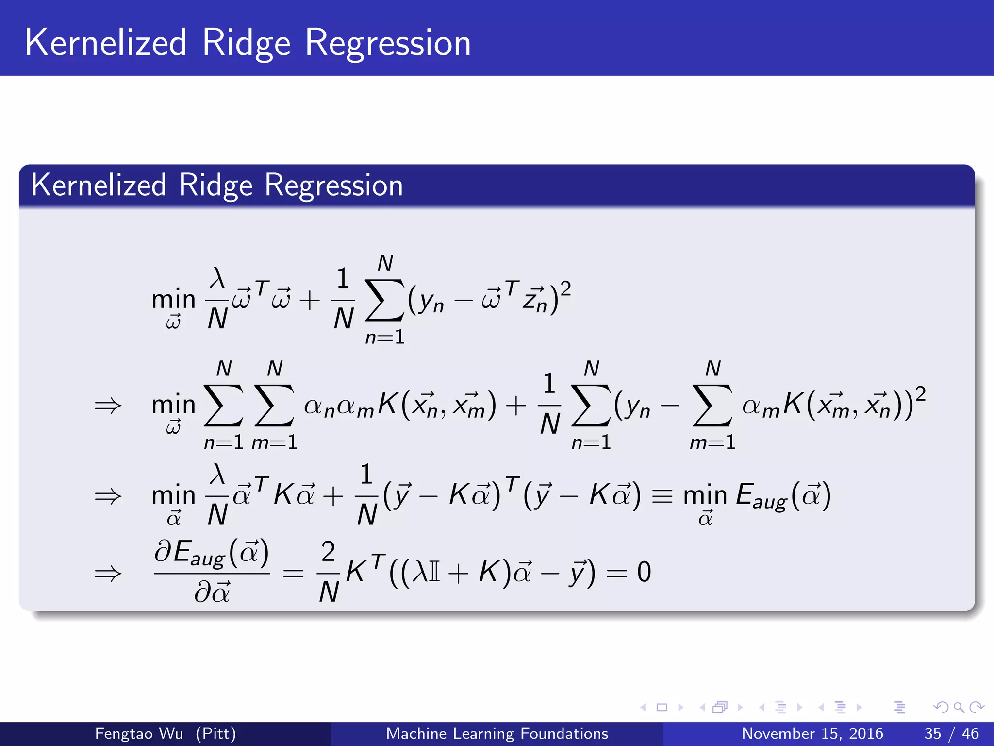
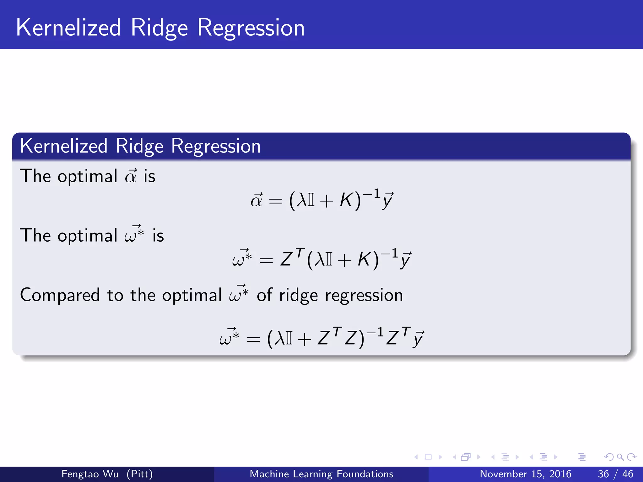
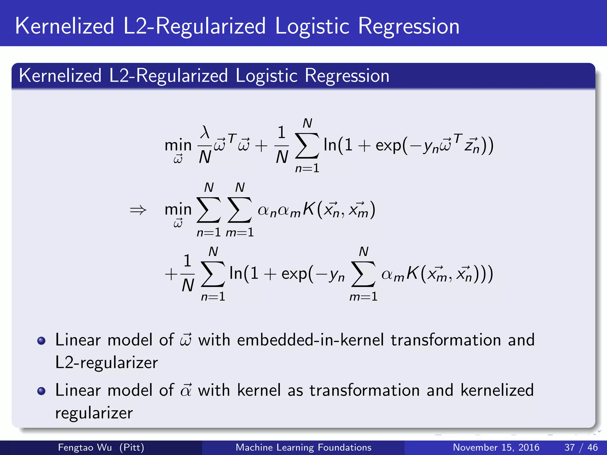
Discusses kernelized forms of linear models, focusing on Ridge, Logistic Regression, and their unique formulations.
Introduces Tube Regression and its L2-Regularized variant, drawing parallels to Soft-Margin SVM.
Describes components, constraints, and optimization techniques for Support Vector Regression models.
Lists reference materials utilized throughout the presentation and concludes with a Q&A session.


![[DSC Europe 25] Dragan Vucic - Building the Learning Organization - How AI Tr...](https://cdn.slidesharecdn.com/ss_thumbnails/8brigo2sbu6qur6gxrra-7-251205085715-6ae07d24-thumbnail.jpg?width=640&height=640&fit=bounds)


![[DSC Europe 25] Max Talanov - Non digital NNs.pptx](https://cdn.slidesharecdn.com/ss_thumbnails/wif8tr3gtua74qvtopke-non-digital-nns-251205090438-26b0eea6-thumbnail.jpg?width=640&height=640&fit=bounds)
![[DSC Europe 25] Dusan Jovicic - AI Story: From on-prem to cloud and back agai...](https://cdn.slidesharecdn.com/ss_thumbnails/8kp49m6uq22ifnbwhfnk-2-251205085715-964d11a6-thumbnail.jpg?width=640&height=640&fit=bounds)


![[DSC Europe 25] Petar Zivanov - AI meets documents From chatbots to AI-powere...](https://cdn.slidesharecdn.com/ss_thumbnails/xer2bb6nrdc8pdpev0pc-8-251204082258-7c2fa4a1-thumbnail.jpg?width=640&height=640&fit=bounds)


![[DSC Europe 25] Dragana Ilic - AI for Big Data in Astronomy.pptx](https://cdn.slidesharecdn.com/ss_thumbnails/8palya86qaatvjhva1ms-2-dragana-ilic-ai-ilic-251208151906-652b819c-thumbnail.jpg?width=640&height=640&fit=bounds)

