Download to read offline

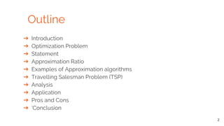

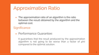
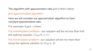
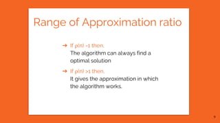
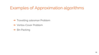

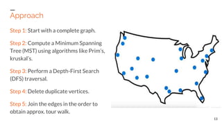
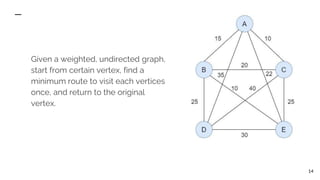
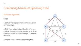


The document discusses approximation algorithms, which are efficient methods for finding near-optimal solutions to NP-hard optimization problems when exact solutions are impractical. It details the concept of approximation ratios, examples like the Traveling Salesman Problem, and the steps involved in constructing algorithms to ensure performance guarantees. The conclusion highlights that approximation algorithms aim to achieve close-to-optimal results within polynomial time frames, though they may not always provide the best solution.


![Attack surfaces and attack tress[inform]](https://cdn.slidesharecdn.com/ss_thumbnails/lecture03-260108015941-a4dee53b-thumbnail.jpg?width=640&height=640&fit=bounds)


