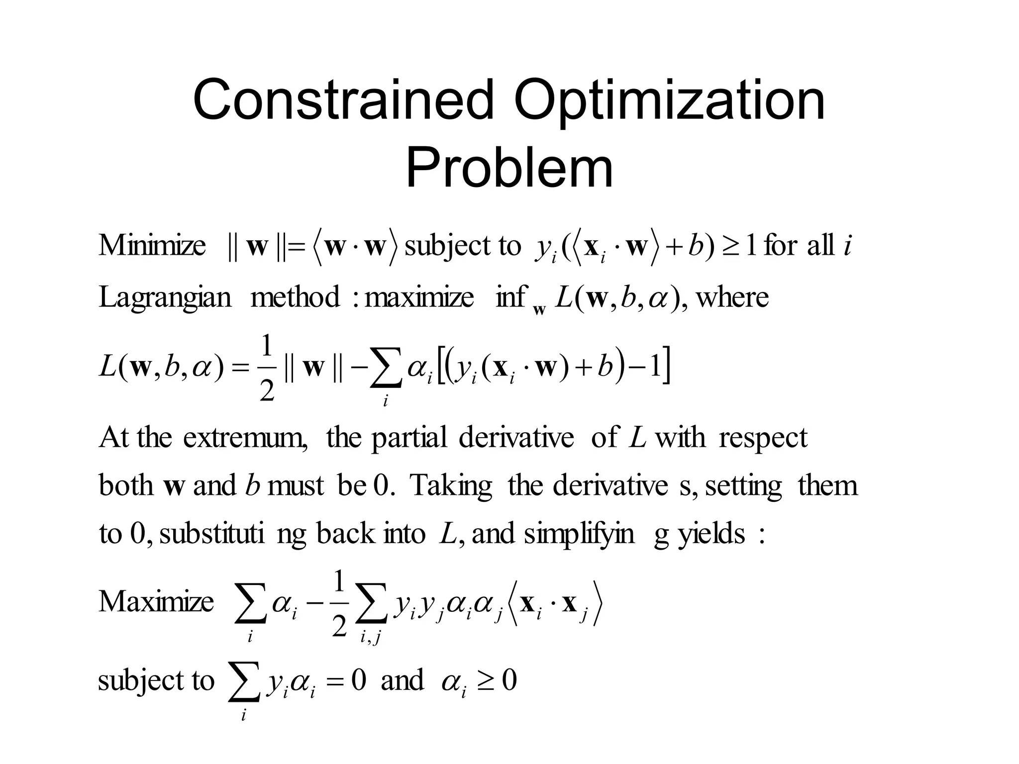
This document provides an introduction to support vector machines (SVMs). It discusses key concepts such as using a max-margin classifier to find the optimal separating hyperplane, using Lagrangian multipliers to solve constrained optimization problems, projecting data into higher dimensions to make it linearly separable, and how complexity depends on training examples rather than dimensionality. It also covers examples of using SVMs for classification tasks like protein localization and discusses overfitting issues.

1. An Introduction to Support Vector
Machines
CSE 573 Autumn 2005
Henry Kautz
based on slides stolen from Pierre Dönnes’ web site

2. Main Ideas
• Max-Margin Classifier
– Formalize notion of the best linear separator
• Lagrangian Multipliers
– Way to convert a constrained optimization problem
to one that is easier to solve
• Kernels
– Projecting data into higher-dimensional space
makes it linearly separable
• Complexity
– Depends only on the number of training examples,
not on dimensionality of the kernel space!

3. Tennis example
Humidity
Temperature
= play tennis
= do not play tennis

4. Linear Support Vector
Machines
x1
x2
=+1
=-1
Data: <xi,yi>, i=1,..,l
xi  Rd
yi  {-1,+1}

5. =-1
=+1
Data: <xi,yi>, i=1,..,l
xi  Rd
yi  {-1,+1}
All hyperplanes in Rd are parameterize by a vector (w) and a constant b.
Can be expressed as w•x+b=0 (remember the equation for a hyperplane
from algebra!)
Our aim is to find such a hyperplane f(x)=sign(w•x+b), that
correctly classify our data.
f(x)
Linear SVM 2

6. d+
d-
Definitions
Define the hyperplane H such that:
xi•w+b  +1 when yi =+1
xi•w+b  -1 when yi =-1
d+ = the shortest distance to the closest positive point
d- = the shortest distance to the closest negative point
The margin of a separating hyperplane is d+ + d-.
H
H1 and H2 are the planes:
H1: xi•w+b = +1
H2: xi•w+b = -1
The points on the planes
H1 and H2 are the
Support Vectors
H1
H2

7. Maximizing the margin
d+
d-
We want a classifier with as big margin as possible.
Recall the distance from a point(x0,y0) to a line:
Ax+By+c = 0 is|A x0 +B y0 +c|/sqrt(A2+B2)
The distance between H and H1 is:
|w•x+b|/||w||=1/||w||
The distance between H1 and H2 is: 2/||w||
In order to maximize the margin, we need to minimize ||w||. With the
condition that there are no datapoints between H1 and H2:
xi•w+b  +1 when yi =+1
xi•w+b  -1 when yi =-1 Can be combined into yi(xi•w)  1
H1
H2
H

8. Constrained Optimization
Problem
 
 
0
and
0
subject to
2
1
Maximize
:
yields
g
simplifyin
and
,
into
back
ng
substituti
0,
to
them
setting
s,
derivative
the
Taking
0.
be
must
and
both
respect
with
of
derivative
partial
the
extremum,
At the
1
)
(
||
||
2
1
)
,
,
(
where
,
)
,
,
(
inf
maximize
:
method
Lagrangian
all
for
1
)
(
subject to
||
||
Minimize
,















 

i
i
i
i
i j
i
j
i
j
i
j
i
i
i
i
i
i
i
i
y
y
y
L
b
L
b
y
b
L
b
L
i
b
y








x
x
w
w
x
w
w
w
w
x
w
w
w
w

9. Quadratic Programming
• Why is this reformulation a good thing?
• The problem
is an instance of what is called a positive, semi-definite
programming problem
• For a fixed real-number accuracy, can be solved in
O(n log n) time = O(|D|2 log |D|2)
0
and
0
subject to
2
1
Maximize
,





 
i
i
i
i
i j
i
j
i
j
i
j
i
i
y
y
y




 x
x

10. Problems with linear SVM
=-1
=+1
What if the decision function is not a linear?

11. Kernel Trick
)
2
,
,
(
space
in the
separable
linearly
are
points
Data
2
1
2
2
2
1 x
x
x
x
2
,
)
,
(
Here,
directly!
compute
easy to
often
is
:
thing
Cool
)
(
)
(
)
,
(
Define
)
(
)
(
2
1
maximize
want to
We
j
i
j
i
j
i
j
i
i j
i
j
i
j
i
j
i
i
K
K
F
F
K
F
F
y
y
x
x
x
x
x
x
x
x
x
x






  



12. Other Kernels
The polynomial kernel
K(xi,xj) = (xi•xj + 1)p, where p is a tunable parameter.
Evaluating K only require one addition and one exponentiation
more than the original dot product.
Gaussian kernels (also called radius basis functions)
K(xi,xj) = exp(||xi-xj ||2/22)

13. Overtraining/overfitting
=-1
=+1
An example: A botanist really knowing trees.Everytime he sees a new tree,
he claims it is not a tree.
A well known problem with machine learning methods is overtraining.
This means that we have learned the training data very well, but
we can not classify unseen examples correctly.

14. Overtraining/overfitting 2
It can be shown that: The portion, n, of unseen data that will be
missclassified is bounded by:
n  Number of support vectors / number of training examples
A measure of the risk of overtraining with SVM (there are also other
measures).
Ockham´s razor principle: Simpler system are better than more complex ones.
In SVM case: fewer support vectors mean a simpler representation of the
hyperplane.
Example: Understanding a certain cancer if it can be described by one gene
is easier than if we have to describe it with 5000.

15. A practical example, protein
localization
• Proteins are synthesized in the cytosol.
• Transported into different subcellular
locations where they carry out their
functions.
• Aim: To predict in what location a
certain protein will end up!!!

16. Subcellular Locations

17. Method
• Hypothesis: The amino acid composition of proteins
from different compartments should differ.
• Extract proteins with know subcellular location from
SWISSPROT.
• Calculate the amino acid composition of the proteins.
• Try to differentiate between: cytosol, extracellular,
mitochondria and nuclear by using SVM

18. Input encoding
Prediction of nuclear proteins:
Label the known nuclear proteins as +1 and all others
as –1.
The input vector xi represents the amino acid
composition.
Eg xi =(4.2,6.7,12,….,0.5)
A , C , D,….., Y)
Nuclear
All others
SVM Model

19. Cross-validation
Cross validation: Split the data into n sets, train on n-1 set, test on the set left
out of training.
Nuclear
All others
1
2
3
1
2
3
Test set
1
1
Training set
2
3
2
3

20. Performance measurments
Model
=+1
=-1
Predictions
+1
-1
Test data TP
FP
TN
FN
SP = TP /(TP+FP), the fraction of predicted +1 that actually are +1.
SE = TP /(TP+FN), the fraction of the +1 that actually are predicted as +1.
In this case: SP=5/(5+1) =0.83
SE = 5/(5+2) = 0.71

21. A Cautionary Example
Image classification of tanks. Autofire when an enemy tank is spotted.
Input data: Photos of own and enemy tanks.
Worked really good with the training set used.
In reality it failed completely.
Reason: All enemy tank photos taken in the morning. All own tanks in dawn.
The classifier could recognize dusk from dawn!!!!

22. References
http://www.kernel-machines.org/
AN INTRODUCTION TO SUPPORT VECTOR MACHINES
(and other kernel-based learning methods)
N. Cristianini and J. Shawe-Taylor
Cambridge University Press
2000 ISBN: 0 521 78019 5
http://www.support-vector.net/
Papers by Vapnik
C.J.C. Burges: A tutorial on Support Vector Machines. Data Mining and
Knowledge Discovery 2:121-167, 1998.