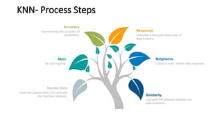
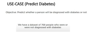
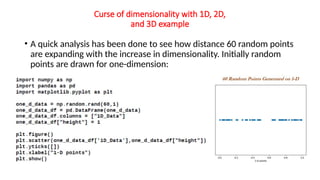
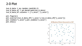
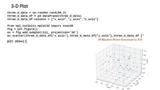
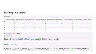
SML
UNIT-3
K-Nearest Neighbors
K-nearest neighbors (KNN) algorithm
is a type of supervised ML algorithm which can be used for both
classification as well as regression predictive problems.
However, it is mainly used for classification predictive problems in
industry. The following two properties would define KNN well
• Lazy learning algorithm − KNN is a lazy learning algorithm because it
does not have a specialized training phase and uses all the data for
training while classification.
• Non-parametric learning algorithm − KNN is also a non-parametric
learning algorithm because it doesn’t assume anything about the
underlying data.
K-Nearest Neighbors
The K-NN working can be explained on the basis of the below
algorithm:
• Step-1: Select the number K of the neighbors
• Step-2: Calculate the Euclidean distance of K number of neighbors
• Step-3: Take the K nearest neighbors as per the calculated Euclidean
distance.
• Step-4: Among these k neighbors, count the number of the data
points in each category.
• Step-5: Assign the new data points to that category for which the
number of the neighbor is maximum.
• Step-6: Our model is ready.
Working process of KNN Algorithm
• K-nearest neighbors (KNN) algorithm uses ‘feature similarity’ to predict the
values of new data points which further means that the new data point will
be assigned a value based on how closely it matches the points in the
training set.
• We can understand its working with the help of following steps −
Step 1 − For implementing any algorithm, we need dataset. So during
the first step of KNN, we must load the training as well as test data.
Step 2 − Next, we need to choose the value of K i.e. the nearest data
points. K can be any integer.
Working process of KNN Algorithm
Step 3 − For each point in the test data do the following −
3.1 − Calculate the distance between test data and each row of
training data with the help of any of the method namely: Euclidean,
Manhattan or Hamming distance. The most commonly used method to
calculate distance is Euclidean.
3.2 − Now, based on the distance value, sort them in ascending
order.
3.3 − Next, it will choose the top K rows from the sorted array.
3.4 − Now, it will assign a class to the test point based on most
frequent class of these rows.
Step 4 − End
• Now, we need to classify new data point with black dot (at point
60,60) into blue or red class. We are assuming K = 3 i.e. it would find
three nearest data points. It is shown in the next diagram
Working of KNN Algorithm with concept of K
KNN-Simple Example
• Suppose, we have an image of a creature that looks similar to cat and dog,
but we want to know either it is a cat or dog.
• So for this identification, we can use the KNN algorithm, as it works on a
similarity measure.
• Our KNN model will find the similar features of the new data set to the cats
and dogs images and based on the most similar features it will put it in either
cat or dog category.
Advantages of KNN
• It is very simple algorithm to understand and interpret.
• It is very useful for nonlinear data because there is no assumption about data
in this algorithm.
• It is a versatile algorithm as we can use it for classification as well as
regression.
• It has relatively high accuracy but there are much better supervised learning
models than KNN.
Disadvantages of KNN
• It is computationally a bit expensive algorithm because it stores all the
training data.
• High memory storage required as compared to other supervised learning
algorithms.
• Prediction is slow in case of big N.
• It is very sensitive to the scale of data as well as irrelevant features.
Applications of KNN
The following are some of the areas in which KNN can be applied successfully
Banking System
• KNN can be used in banking system to predict weather an individual is fit for loan
approval?
• Does that individual have the characteristics similar to the defaulters one?
Calculating Credit Ratings
• KNN algorithms can be used to find an individual’s credit rating by comparing with
the persons having similar traits.
Politics
• With the help of KNN algorithms, we can classify a potential voter into various
classes like “Will Vote”, “Will not Vote”, “Will Vote to Party ‘Congress’, “Will Vote
to Party ‘BJP’.
• Other areas in which KNN algorithm can be used are Speech Recognition,
Handwriting Detection, Image Recognition and Video Recognition.
KNN voter example
• Objective is to predict the party for which voter will vote based on their
neighborhood, precisely geolocation (latitude and longitude).
• Here we assume that we can identify the potential voter to which political
party they would be voting based on majority voters did voted for that
particular party in that vicinity, so that they have high probability to vote for
the majority party.
• However,
tuning the k-value
(number to consider, among which majority should be counted)
is the milliondollar question
(as same as any machine learning algorithm):
KNN voter example
KNN voter example
• Party 2- As within the vicinity, one neighbor has voted for Party 1 and
the other voter voted for Party 3.
• But three voters voted for Party 2.
• In fact, by this way KNN solves any given classification problem.
• Regression problems are solved by taking mean of its neighbors within
the given circle or vicinity or k-value.
How does KNN Algorithm works ?
KNN- Example:
KNN- Example:
KNN- IRIS (Dataset)
KNN- Process Steps
USE-CASE (Predict Diabetes)
Diabetes- Dataset
Implementation- Predict Diabetes
Import Libraries
Load Dataset
Load Dataset
List out Glucose Feature in a Dataset
KNN Classifier Model
Predict Test
Evaluate Model
F1 Score and Accuracy
Curse of dimensionality
• KNN completely depends on distance.
• Studying about the curse of dimensionality to understand when KNN
deteriorates its predictive power with the increase in number of variables
required for prediction.
• Though there are many ways to check the curve of dimensionality, here we
are using uniform random values between zero and one generated for 1D,
2D, and 3D space to validate this hypothesis.
• mean distance between 1,000 observations have been calculated with the
change in dimensions.
• increase in dimensions, distance between points increases logarithmically,
which gives us the hint that we need to have exponential increase in data
points with increase in dimensions in order to make machine learning
algorithms
Curse of dimensionality
• mean distance between 1,000 observations have been calculated with the
change in dimensions.
• It is apparent that with the increase in dimensions, distance between points
increases logarithmically, which gives us the hint that we need to have
exponential increase in data points with increase in dimensions in order to
make machine learning algorithms work correctly:
Curse of dimensionality
Curse of dimensionality with 1D, 2D,
and 3D example
• A quick analysis has been done to see how distance 60 random points
are expanding with the increase in dimensionality. Initially random
points are drawn for one-dimension:
2-D Plot
3-D Plot
KNN-Predictions
knnPredictions=pd.DataFrame(predicted_1)
df1=pd.([knnPredictions], axis =1)
df1
Naive Bayes
• Foundational mathematical principles for determining the probability of
unknown events from the known events.
• Example:
if all apples are red in color and average diameter would be about 4
inches then, if at random one fruit is selected from the basket with red color
and diameter of 3.7 inch
what is the probability that the particular fruit would be an apple?
here would be no dependency between color and diameter.
• independence assumption makes the Naive Bayes classifier most effective in
terms of computational ease for particular tasks such as email classification
based on words in which high dimensions of vocab do exist, even after
assuming independence between features.
Naive Bayes
• Bayesian classifiers are best applied to problems in which information from a
very high number of attributes should be considered simultaneously to
estimate the probability of final outcome.
• Bayesian methods utilize all available evidence to consider for prediction
even features have weak effects on the final outcome to predict.
• However, we should not ignore the fact that a large number of features with
relatively minor effects, taken together its combined impact would form
strong classifiers
Probability Fundamentals
• Probability of an event can be estimated from observed data by
dividing the number of trails in which an event occurred with total
number of trails.
• If a bag contains red and blue balls and randomly picked 10 balls one
by one with replacement and out of 10, 3 red balls appeared in trails
we can say that probability of red is 0.3,
pred = 3/10 = 0.3.
Total probability of all possible outcomes must be 100 percent.
Probability Fundamentals
• If a trail has two outcomes such as email classification either it is spam
or not spam and both cannot occur simultaneously, these events are
considered as mutually exclusive with each other.
• In addition, if those outcomes cover all possible events, it would be
called as exhaustive events.
For example,
In Email classification if P (spam) = 0.1.
• we will be able to calculate P (ham) = 1- 0.1 = 0.9, these two events are
mutually exclusive. In the following Venn diagram, all the email possible
classes are represented (the entire universe) with type of outcomes.
Probability Fundamentals
• For example, in email
• classification if P (spam) = 0.1, we will be able to calculate P (ham) =
1- 0.1 = 0.9, these two events are mutually exclusive.
• In the following Venn diagram, all the email possible classes are
represented (the entire universe) with type of outcomes:
Joint probability
• Though mutually exclusive cases are simple to work upon, most of the actual
problems do fall under the category of non-mutually exclusive events.
• By using the joint appearance, we can predict the event outcome.
• Example:
if emails messages present the word like lottery, which is very highly
likely of being spam rather than ham.
Joint probability
• The following Venn diagram indicates the joint probability of spam with
lottery.
• However, if you notice in detail, lottery circle is not contained
completely within the spam circle.
• This implies that not all spam messages contain the word lottery and
not every email with the word lottery is spam.
Joint probability
• In case if both the events are totally unrelated, they are called
independent events and their respective value is
• p(spam ∩ lottery) = p(spam) * p(lottery) = 0.1 * 0.04 = 0.004,
which is 0.4 percent of all messages are spam containing the word
Lottery.
In general, for independent events P(A∩ B) = P(A)* P(B).
Understanding Bayes theorem with
conditional probability
• Conditional probability provides a way of calculating relationships
between dependent events using Bayes theorem
• For example, A and B are two events and
• we would like to calculate P(AB) can be read as the probability of
event occurring A given the fact that event B already occurred, in fact
this is known as conditional probability
Understanding Bayes theorem with
conditional probability
• we will now talk about the email classification example.
• Our objective is to predict whether email is spam given the word
lottery and some other clues.
• In this case we already knew the overall probability of spam, which is
10 percent also known as prior probability.
• Now suppose you have obtained an additional piece of information
that probability of word lottery in all messages, which is 4 percent,
also known as marginal likelihood
Understanding Bayes theorem with
conditional probability
• We know the probability that lottery was used in previous spam
messages and is called the likelihood.
Understanding Bayes theorem with
conditional probability
Naive Bayes classification
• Let us construct the likelihood table for the appearance of the three
words (W1, W2, and W3), as shown in the following table for 100
emails:
Naive Bayes classification
Problem 1 Consider a set of patients coming for treatment in a certain clinic. Let
A denote the event that a “Patient has liver disease” and B the event that a
“Patient is an alcoholic.” It is known from experience that 10% of the patients
entering the clinic have liver disease and 5% of the patients are alcoholics. Also,
among those patients diagnosed with liver disease, 7% are alcoholics. Given that
a patient is alcoholic, what is the probability that he will have liver disease?
Solution Using the notations of probability, we have
P(A) = 10% = 0.10
P(B) = 5% = 0.05
P(B A) = 7% = 0.07
∣
P(A B) = P(B A)P(A)
∣ ∣
P(B) = 0.07 × 0.10 0.05 = 0.14
Naive Bayes classification
Problem 2 Three factories A, B, C of an electric bulb manufacturing company
produce respectively 35%. 35% and 30% of the total output. Approximately
1.5%, 1% and 2% of the bulbs produced by these factories are known to be
defective. If a randomly selected bulb manufactured by the company was
found to be defective, what is the probability that the bulb was manufactures
in factory A?
Naive Bayes classification

Statistical Machine Learning unit3 lecture notes

  • 1.
  • 2.
    K-Nearest Neighbors K-nearest neighbors(KNN) algorithm is a type of supervised ML algorithm which can be used for both classification as well as regression predictive problems. However, it is mainly used for classification predictive problems in industry. The following two properties would define KNN well • Lazy learning algorithm − KNN is a lazy learning algorithm because it does not have a specialized training phase and uses all the data for training while classification. • Non-parametric learning algorithm − KNN is also a non-parametric learning algorithm because it doesn’t assume anything about the underlying data.
  • 3.
    K-Nearest Neighbors The K-NNworking can be explained on the basis of the below algorithm: • Step-1: Select the number K of the neighbors • Step-2: Calculate the Euclidean distance of K number of neighbors • Step-3: Take the K nearest neighbors as per the calculated Euclidean distance. • Step-4: Among these k neighbors, count the number of the data points in each category. • Step-5: Assign the new data points to that category for which the number of the neighbor is maximum. • Step-6: Our model is ready.
  • 4.
    Working process ofKNN Algorithm • K-nearest neighbors (KNN) algorithm uses ‘feature similarity’ to predict the values of new data points which further means that the new data point will be assigned a value based on how closely it matches the points in the training set. • We can understand its working with the help of following steps − Step 1 − For implementing any algorithm, we need dataset. So during the first step of KNN, we must load the training as well as test data. Step 2 − Next, we need to choose the value of K i.e. the nearest data points. K can be any integer.
  • 5.
    Working process ofKNN Algorithm Step 3 − For each point in the test data do the following − 3.1 − Calculate the distance between test data and each row of training data with the help of any of the method namely: Euclidean, Manhattan or Hamming distance. The most commonly used method to calculate distance is Euclidean. 3.2 − Now, based on the distance value, sort them in ascending order. 3.3 − Next, it will choose the top K rows from the sorted array. 3.4 − Now, it will assign a class to the test point based on most frequent class of these rows. Step 4 − End
  • 6.
    • Now, weneed to classify new data point with black dot (at point 60,60) into blue or red class. We are assuming K = 3 i.e. it would find three nearest data points. It is shown in the next diagram Working of KNN Algorithm with concept of K
  • 7.
    Working of KNNAlgorithm with concept of K
  • 8.
    KNN-Simple Example • Suppose,we have an image of a creature that looks similar to cat and dog, but we want to know either it is a cat or dog. • So for this identification, we can use the KNN algorithm, as it works on a similarity measure. • Our KNN model will find the similar features of the new data set to the cats and dogs images and based on the most similar features it will put it in either cat or dog category.
  • 9.
    Advantages of KNN •It is very simple algorithm to understand and interpret. • It is very useful for nonlinear data because there is no assumption about data in this algorithm. • It is a versatile algorithm as we can use it for classification as well as regression. • It has relatively high accuracy but there are much better supervised learning models than KNN.
  • 10.
    Disadvantages of KNN •It is computationally a bit expensive algorithm because it stores all the training data. • High memory storage required as compared to other supervised learning algorithms. • Prediction is slow in case of big N. • It is very sensitive to the scale of data as well as irrelevant features.
  • 11.
    Applications of KNN Thefollowing are some of the areas in which KNN can be applied successfully Banking System • KNN can be used in banking system to predict weather an individual is fit for loan approval? • Does that individual have the characteristics similar to the defaulters one? Calculating Credit Ratings • KNN algorithms can be used to find an individual’s credit rating by comparing with the persons having similar traits. Politics • With the help of KNN algorithms, we can classify a potential voter into various classes like “Will Vote”, “Will not Vote”, “Will Vote to Party ‘Congress’, “Will Vote to Party ‘BJP’. • Other areas in which KNN algorithm can be used are Speech Recognition, Handwriting Detection, Image Recognition and Video Recognition.
  • 12.
    KNN voter example •Objective is to predict the party for which voter will vote based on their neighborhood, precisely geolocation (latitude and longitude). • Here we assume that we can identify the potential voter to which political party they would be voting based on majority voters did voted for that particular party in that vicinity, so that they have high probability to vote for the majority party. • However, tuning the k-value (number to consider, among which majority should be counted) is the milliondollar question (as same as any machine learning algorithm):
  • 13.
  • 14.
    KNN voter example •Party 2- As within the vicinity, one neighbor has voted for Party 1 and the other voter voted for Party 3. • But three voters voted for Party 2. • In fact, by this way KNN solves any given classification problem. • Regression problems are solved by taking mean of its neighbors within the given circle or vicinity or k-value.
  • 15.
    How does KNNAlgorithm works ?
  • 16.
    How does KNNAlgorithm works ?
  • 17.
    How does KNNAlgorithm works ?
  • 18.
  • 19.
  • 20.
  • 21.
  • 22.
  • 23.
  • 24.
  • 25.
  • 26.
  • 27.
  • 29.
    List out GlucoseFeature in a Dataset
  • 33.
  • 34.
  • 35.
  • 36.
    F1 Score andAccuracy
  • 37.
    Curse of dimensionality •KNN completely depends on distance. • Studying about the curse of dimensionality to understand when KNN deteriorates its predictive power with the increase in number of variables required for prediction. • Though there are many ways to check the curve of dimensionality, here we are using uniform random values between zero and one generated for 1D, 2D, and 3D space to validate this hypothesis. • mean distance between 1,000 observations have been calculated with the change in dimensions. • increase in dimensions, distance between points increases logarithmically, which gives us the hint that we need to have exponential increase in data points with increase in dimensions in order to make machine learning algorithms
  • 38.
    Curse of dimensionality •mean distance between 1,000 observations have been calculated with the change in dimensions. • It is apparent that with the increase in dimensions, distance between points increases logarithmically, which gives us the hint that we need to have exponential increase in data points with increase in dimensions in order to make machine learning algorithms work correctly:
  • 39.
  • 40.
  • 41.
    Curse of dimensionalitywith 1D, 2D, and 3D example • A quick analysis has been done to see how distance 60 random points are expanding with the increase in dimensionality. Initially random points are drawn for one-dimension:
  • 42.
  • 43.
  • 48.
  • 52.
    Naive Bayes • Foundationalmathematical principles for determining the probability of unknown events from the known events. • Example: if all apples are red in color and average diameter would be about 4 inches then, if at random one fruit is selected from the basket with red color and diameter of 3.7 inch what is the probability that the particular fruit would be an apple? here would be no dependency between color and diameter. • independence assumption makes the Naive Bayes classifier most effective in terms of computational ease for particular tasks such as email classification based on words in which high dimensions of vocab do exist, even after assuming independence between features.
  • 53.
    Naive Bayes • Bayesianclassifiers are best applied to problems in which information from a very high number of attributes should be considered simultaneously to estimate the probability of final outcome. • Bayesian methods utilize all available evidence to consider for prediction even features have weak effects on the final outcome to predict. • However, we should not ignore the fact that a large number of features with relatively minor effects, taken together its combined impact would form strong classifiers
  • 54.
    Probability Fundamentals • Probabilityof an event can be estimated from observed data by dividing the number of trails in which an event occurred with total number of trails. • If a bag contains red and blue balls and randomly picked 10 balls one by one with replacement and out of 10, 3 red balls appeared in trails we can say that probability of red is 0.3, pred = 3/10 = 0.3. Total probability of all possible outcomes must be 100 percent.
  • 55.
    Probability Fundamentals • Ifa trail has two outcomes such as email classification either it is spam or not spam and both cannot occur simultaneously, these events are considered as mutually exclusive with each other. • In addition, if those outcomes cover all possible events, it would be called as exhaustive events. For example, In Email classification if P (spam) = 0.1. • we will be able to calculate P (ham) = 1- 0.1 = 0.9, these two events are mutually exclusive. In the following Venn diagram, all the email possible classes are represented (the entire universe) with type of outcomes.
  • 56.
    Probability Fundamentals • Forexample, in email • classification if P (spam) = 0.1, we will be able to calculate P (ham) = 1- 0.1 = 0.9, these two events are mutually exclusive. • In the following Venn diagram, all the email possible classes are represented (the entire universe) with type of outcomes:
  • 58.
    Joint probability • Thoughmutually exclusive cases are simple to work upon, most of the actual problems do fall under the category of non-mutually exclusive events. • By using the joint appearance, we can predict the event outcome. • Example: if emails messages present the word like lottery, which is very highly likely of being spam rather than ham.
  • 59.
    Joint probability • Thefollowing Venn diagram indicates the joint probability of spam with lottery. • However, if you notice in detail, lottery circle is not contained completely within the spam circle. • This implies that not all spam messages contain the word lottery and not every email with the word lottery is spam.
  • 61.
    Joint probability • Incase if both the events are totally unrelated, they are called independent events and their respective value is • p(spam ∩ lottery) = p(spam) * p(lottery) = 0.1 * 0.04 = 0.004, which is 0.4 percent of all messages are spam containing the word Lottery. In general, for independent events P(A∩ B) = P(A)* P(B).
  • 62.
    Understanding Bayes theoremwith conditional probability • Conditional probability provides a way of calculating relationships between dependent events using Bayes theorem • For example, A and B are two events and • we would like to calculate P(AB) can be read as the probability of event occurring A given the fact that event B already occurred, in fact this is known as conditional probability
  • 63.
    Understanding Bayes theoremwith conditional probability • we will now talk about the email classification example. • Our objective is to predict whether email is spam given the word lottery and some other clues. • In this case we already knew the overall probability of spam, which is 10 percent also known as prior probability. • Now suppose you have obtained an additional piece of information that probability of word lottery in all messages, which is 4 percent, also known as marginal likelihood
  • 64.
    Understanding Bayes theoremwith conditional probability • We know the probability that lottery was used in previous spam messages and is called the likelihood.
  • 65.
    Understanding Bayes theoremwith conditional probability
  • 66.
    Naive Bayes classification •Let us construct the likelihood table for the appearance of the three words (W1, W2, and W3), as shown in the following table for 100 emails:
  • 67.
    Naive Bayes classification Problem1 Consider a set of patients coming for treatment in a certain clinic. Let A denote the event that a “Patient has liver disease” and B the event that a “Patient is an alcoholic.” It is known from experience that 10% of the patients entering the clinic have liver disease and 5% of the patients are alcoholics. Also, among those patients diagnosed with liver disease, 7% are alcoholics. Given that a patient is alcoholic, what is the probability that he will have liver disease? Solution Using the notations of probability, we have P(A) = 10% = 0.10 P(B) = 5% = 0.05 P(B A) = 7% = 0.07 ∣ P(A B) = P(B A)P(A) ∣ ∣ P(B) = 0.07 × 0.10 0.05 = 0.14
  • 68.
    Naive Bayes classification Problem2 Three factories A, B, C of an electric bulb manufacturing company produce respectively 35%. 35% and 30% of the total output. Approximately 1.5%, 1% and 2% of the bulbs produced by these factories are known to be defective. If a randomly selected bulb manufactured by the company was found to be defective, what is the probability that the bulb was manufactures in factory A?
  • 69.
  • 70.
  • 71.
  • 72.
  • 73.
  • 74.
  • 75.
  • 76.
  • 77.