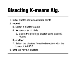
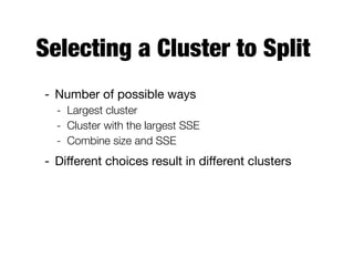
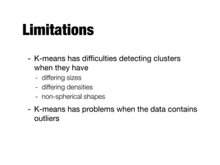
Download as PDF, PPTX


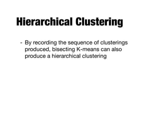
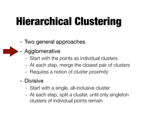
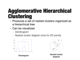
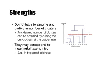
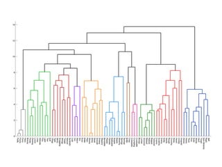
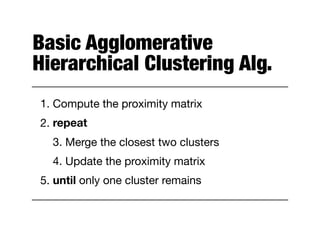
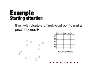
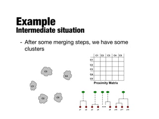
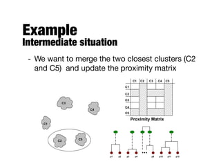
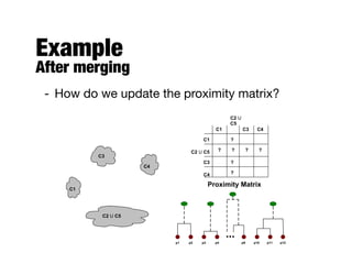


Hierarchical clustering builds clusters hierarchically, by either merging or splitting clusters at each step. Agglomerative hierarchical clustering starts with each point as a separate cluster and successively merges the closest clusters based on a defined proximity measure between clusters. This results in a dendrogram showing the nested clustering structure. The basic algorithm computes a proximity matrix, then repeatedly merges the closest pair of clusters and updates the matrix until all points are in one cluster.


![Chapter#04[Part#01]K-Means Clusterig.pdf](https://cdn.slidesharecdn.com/ss_thumbnails/chapter04part01k-meansclusterig-250525201708-2d369307-thumbnail.jpg?width=640&height=640&fit=bounds)


![[ML]-Unsupervised-learning_Unit2.ppt.pdf](https://cdn.slidesharecdn.com/ss_thumbnails/ml-unsupervised-learningunit2-230916145038-acbd0397-thumbnail.jpg?width=640&height=640&fit=bounds)