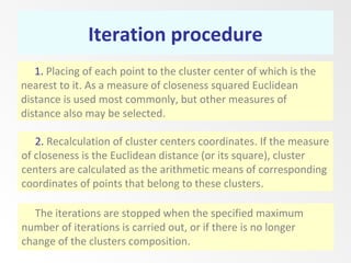
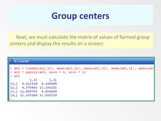
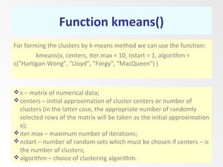
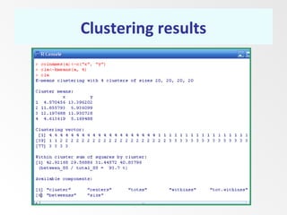
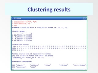
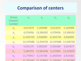
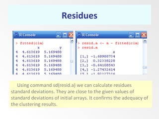
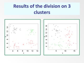
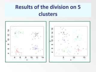
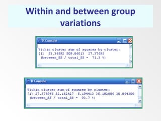
Cluster analysis using k-means
method
Vladimir Bakhrushin,
Professor, D.Sc. (Phys. & Math.)
Vladimir.Bakhrushin@gmail.com
Formulation of the problem
The task of cluster analysis is to divide the existing set of
points on a certain number of groups (clusters) so that the sum
of squares of points distances from cluster centers was minimal.
At the point of minimum all cluster centers coincide with the
centers of the corresponding areas of Voronoi diagram.
Main algorithms:
Hartigan and Wong Lloyd
Lloyd-Forgy MacQueen
The initial approximation
First step is to set the initial approximation of cluster centers.
To do this, such methods are most commonly used:
 to set the centers of clusters directly;
 to set the number of clusters k and take the first k
points coordinates as centers;
 to set the number of clusters k and take the
randomly selected k points coordinates as centers (it is
appropriate to carry out calculations for several
random runs of the algorithm).
Iteration procedure
1. Placing of each point to the cluster center of which is the
nearest to it. As a measure of closeness squared Euclidean
distance is used most commonly, but other measures of
distance also may be selected.
2. Recalculation of cluster centers coordinates. If the measure
of closeness is the Euclidean distance (or its square), cluster
centers are calculated as the arithmetic means of corresponding
coordinates of points that belong to these clusters.
The iterations are stopped when the specified maximum
number of iterations is carried out, or if there is no longer
change of the clusters composition.
Limitation
(shortcoming)
Setting the
number of
clusters (initial
approximation)
Preliminary analysis
of data
Sensitivity to
outliers
Using of
k-medians
Limitations and shortcomings
Using of random
samples from
arrays
Slow work on large
arrays
Forming of data array
a1 = matrix(c(rnorm(20, mean = 5, sd = 1), rnorm(20, mean = 5,
sd = 1)), nrow=20, ncol = 2)
a2 = matrix(c(rnorm(20, mean = 5, sd = 1), rnorm(20, mean =
13, sd = 1)), nrow=20, ncol = 2)
a3 = matrix(c(rnorm(20, mean = 12, sd = 1), rnorm(20, mean =
6, sd = 1)), nrow=20, ncol = 2)
a4 = matrix(c(rnorm(20, mean = 12, sd = 1), rnorm(20, mean =
12, sd = 1)), nrow=20, ncol = 2)
a <- rbind(a1,a2,a3,a4)
Function rbind() forms matrix a, in which the first 20 rows are the
corresponding strings of matrix a1, next 20 – matrix a2 and so
on.
Group centers
Next, we must calculate the matrix of values of formed group
centers and display the results on a screen:
Function kmeans()
For forming the clusters by k-means method we can use the function:
kmeans(x, centers, iter.max = 10, nstart = 1, algorithm =
c("Hartigan-Wong", "Lloyd", "Forgy", "MacQueen") )
x – matrix of numerical data;
centers – initial approximation of cluster centers or number of
clusters (in the latter case, the appropriate number of randomly
selected rows of the matrix will be taken as the initial approximation
x);
iter.max – maximum number of iterations;
nstart – number of random sets which must be chosen if centers – is
the number of clusters;
algorithm – choice of clustering algorithm.
Clustering results
Clustering results
Clustering results
Comparison of centers
Group
(cluster)
number
xa
ya
xcl
ycl
a1
4,613619 5,169488 4,613619 5,169488
a2
4,570456 13,396202 4,570456 13,396202
a3
11,855793 5,936099 11,855793 5,936099
a4
12,197688 11,930728 12,197688 11,930728
b1
5,531175 5,405187 5,545309 5,527677
b2
5,340795 12,983168 5,472965 13,239925
b3
11,770917 6,725708 11,842934 6,916365
Residues
Using command sd(resid.a) we can calculate residues
standard deviations. They are close to the given values of
standard deviations of initial arrays. It confirms the adequacy of
the clustering results.
Results of the division on 3
clusters
Results of the division on 5
clusters
Within and between group
variations

Cluster analysis using k-means method in R

  • 1.
    Cluster analysis usingk-means method Vladimir Bakhrushin, Professor, D.Sc. (Phys. & Math.) Vladimir.Bakhrushin@gmail.com
  • 2.
    Formulation of theproblem The task of cluster analysis is to divide the existing set of points on a certain number of groups (clusters) so that the sum of squares of points distances from cluster centers was minimal. At the point of minimum all cluster centers coincide with the centers of the corresponding areas of Voronoi diagram. Main algorithms: Hartigan and Wong Lloyd Lloyd-Forgy MacQueen
  • 3.
    The initial approximation Firststep is to set the initial approximation of cluster centers. To do this, such methods are most commonly used:  to set the centers of clusters directly;  to set the number of clusters k and take the first k points coordinates as centers;  to set the number of clusters k and take the randomly selected k points coordinates as centers (it is appropriate to carry out calculations for several random runs of the algorithm).
  • 4.
    Iteration procedure 1. Placingof each point to the cluster center of which is the nearest to it. As a measure of closeness squared Euclidean distance is used most commonly, but other measures of distance also may be selected. 2. Recalculation of cluster centers coordinates. If the measure of closeness is the Euclidean distance (or its square), cluster centers are calculated as the arithmetic means of corresponding coordinates of points that belong to these clusters. The iterations are stopped when the specified maximum number of iterations is carried out, or if there is no longer change of the clusters composition.
  • 5.
    Limitation (shortcoming) Setting the number of clusters(initial approximation) Preliminary analysis of data Sensitivity to outliers Using of k-medians Limitations and shortcomings Using of random samples from arrays Slow work on large arrays
  • 6.
    Forming of dataarray a1 = matrix(c(rnorm(20, mean = 5, sd = 1), rnorm(20, mean = 5, sd = 1)), nrow=20, ncol = 2) a2 = matrix(c(rnorm(20, mean = 5, sd = 1), rnorm(20, mean = 13, sd = 1)), nrow=20, ncol = 2) a3 = matrix(c(rnorm(20, mean = 12, sd = 1), rnorm(20, mean = 6, sd = 1)), nrow=20, ncol = 2) a4 = matrix(c(rnorm(20, mean = 12, sd = 1), rnorm(20, mean = 12, sd = 1)), nrow=20, ncol = 2) a <- rbind(a1,a2,a3,a4) Function rbind() forms matrix a, in which the first 20 rows are the corresponding strings of matrix a1, next 20 – matrix a2 and so on.
  • 7.
    Group centers Next, wemust calculate the matrix of values of formed group centers and display the results on a screen:
  • 8.
    Function kmeans() For formingthe clusters by k-means method we can use the function: kmeans(x, centers, iter.max = 10, nstart = 1, algorithm = c("Hartigan-Wong", "Lloyd", "Forgy", "MacQueen") ) x – matrix of numerical data; centers – initial approximation of cluster centers or number of clusters (in the latter case, the appropriate number of randomly selected rows of the matrix will be taken as the initial approximation x); iter.max – maximum number of iterations; nstart – number of random sets which must be chosen if centers – is the number of clusters; algorithm – choice of clustering algorithm.
  • 9.
  • 10.
  • 11.
  • 12.
    Comparison of centers Group (cluster) number xa ya xcl ycl a1 4,6136195,169488 4,613619 5,169488 a2 4,570456 13,396202 4,570456 13,396202 a3 11,855793 5,936099 11,855793 5,936099 a4 12,197688 11,930728 12,197688 11,930728 b1 5,531175 5,405187 5,545309 5,527677 b2 5,340795 12,983168 5,472965 13,239925 b3 11,770917 6,725708 11,842934 6,916365
  • 13.
    Residues Using command sd(resid.a)we can calculate residues standard deviations. They are close to the given values of standard deviations of initial arrays. It confirms the adequacy of the clustering results.
  • 14.
    Results of thedivision on 3 clusters
  • 15.
    Results of thedivision on 5 clusters
  • 16.
    Within and betweengroup variations