This document summarizes key concepts in condensed matter physics related to interacting electron systems. It introduces the Hartree and Hartree-Fock approximations for modeling interacting electrons, which improve upon treating electrons independently but still do not fully capture electron correlation. The Hartree approximation models the average electrostatic potential felt by each electron from other electrons. Hartree-Fock further includes an "exchange" term to account for the Pauli exclusion principle. It then discusses limitations of these approximations in capturing electron correlation, where the motion of each electron is correlated with all others due to both Coulomb repulsion and the Pauli principle. Capturing electron correlation is important for obtaining more accurate descriptions of materials' properties.

1. 4PHY-3(ii) : CONDENSED MATTER PHYSICS-II
Unit-III
Interacting electron gas, Hartee & Hartee-Fock approximation, Correlation energy, Screening,
dielectric function, Thomas-Fermi and Lindhard Theory, Frequency dependent Lindhard
screening, Screening of Hartee-Fock approximation. Introduction of Fermi Liquid Theory.
Book Referred :
Introduction to Solid State Theory
By Otfried Madelung
Solid State Physics
By N W Ashcroft
&
Introduction to Solid State Physics
By C. Kittel

2. 3.1 Many-Particle Hamiltonians
The Schrodinger equation for a system with more than one particle is
..............1i H
t
 



where H and ψ are the many-particle Hamiltonian and wave function, respectively.
For a set of
non interacting particles, the Hamiltonian of the system is
2
2
( ) .........2
2
i i ii
H H V r
m
 
    
 
 
where the independent-particle solution ψn for each Hi satisfies
2
2
( ) .............3
2
i i n n nV r E
m
 
 
   
 
Now once we consider interaction between electron and electron, lattice ions and
electrons, with equal positive and negative charge. The motion of any particle is now
correlated with all other particles, and such an interacting many-particle system
may be described by the following Hamiltonian
..................4ekin ikin e e e i i iH H H H H H      
Or,
2 2 2
2 2 1 1
( , ) ( , )..........5
2 2 2 2
i i ii i i j i
i j
e
H V r R V R R
m M r r
     
       

    
where ri, m and -e are used to represent the coordinates, mass and charge of
electrons, while Rα, Rβ and M are the corresponding quantities of the lattice ion.
However, it is impossible to solve the Schrodinger equation for the Hamiltonian (5)
in order to have extract solution. Since it is difficult to get results directly, various
approximations and models were introduced with for simplifying the problem.
Under the adiabatic approximation, the coupling between electrons and ions in (5)
is ignored, and we only need to investigate the independent subsystems: one is the
interacting ion system and the other is the interacting electron system . Thus
Hamiltonion for interacting electron system can be written from (5) as,
2 2
2
2 2
2
1
( , )
2 2
simply
1
( ) ..........6
2 2
i ii i j i
i j
i ii i i j
i j
e
H V r R
m r r
or
e
H V r
m r r


    

    

  
  
2
1
, ( )
2 


i i j
i j
e
where V r
r r
Thus Schrodinger equation can be written as,
2 2
2
1 1
1
( ) ( ,.... ) ( ,.... )..........7
2 2
i i N Ni i i j
i j
e
V r r r E r r
m r r
 
 
     
  
  
3.2 The Hartree Approximation
According to hartree the effect of electron-electron interaction on a certain electron ( sat at
r) should be given by electrostatic Coulomb potential generated by all other electrons on
average at position r’. The equation (7) is for interacting electron system.
Thus the total wave function for a system with N electrons could be written as the product
of one-electron wave functions

3. 1
1
( ,.... ) ( )..........8
N
N i i
i
r r r 

 
for which Hartree suggested a variational calculation of E by
| |
.............9
|
H
E
 
 

If ψ were the exact ground state wave functions of the system, then E would be the
ground state energy. Thus it leads to a set of Hartree equations
2
2 2
*( ') ( ')
( ) ' ( ) ( )..........10
2 '
j j
i i ij
r r
V r e dr r E r
m r r
 
 
 
     
 
 
This is the Hartree approximation equation. Where,
2 3
*( ') ( ')
( ) ' the effective potential.
'
 
 

 
j j
eff j
r r
V V r e d r is
r r
where second term represent Hartree potential, which is Coulomb potential between an electron and
average charge density of rest of electron.
Thus in terms of average charge density the potencial can
2 3
be written as
( ')
( ) '
'

Hartree
n r
V r e d r
r r
Where n(r’) is the electron density.
Initially the electron density is not known. For this purpose self consistent field method is
used to calculate n(r’).
And energy eigen values from (9) will be
2
*( ') ( ') *( ) ( )| | 1
'
| 2 '
j j i i
ii i j
r r r rH
E E e drdr
r r
    
  
  

  
The second term is the coulomb interaction energy. If this interaction is dropped from
Hartree equation then the energy of the Hartree electron is purely kinetic as in case of
free electron gas.
The total energy per electron calculated from Hartree energy equation is small
enough to explain metallic cohesion (binding). Thus Hartree approximation needs
modification.
3.3 The Hartree Fock Approximation
The Hartree approximation can be applied to real solids by replacing the original
electron-ion potential by a new one-electron potential . However, to obtain more
realistic interaction, we must go beyond it to introduce the Hartree–Fock
approximation. Because electrons are fermions, the Pauli principle must be
considered. Therefore the total wavefunction for a system with N electrons could be
written as Slater determinant as,
1 1 1
1
( ) ( )
1
( )
( ) ( )
N
i
N N N
r r
r
N
r r
 

 
 
   

   
 
……………………11
The Hartree-Fock approximation can be expressed in terms of the Rayleigh Ritz variational
principle, in which the many-particle wave function is written as a single Slater
determinant.
The Hamiltonian operator is expressed as

4. 𝐻̂ = [∑ −
ħ2
2𝑚
∇2
+ Vions(ri)
𝑖
] +
1
2
∑
𝑒2
| 𝑟𝑖 − 𝑟𝑗|
𝑖≠𝑗
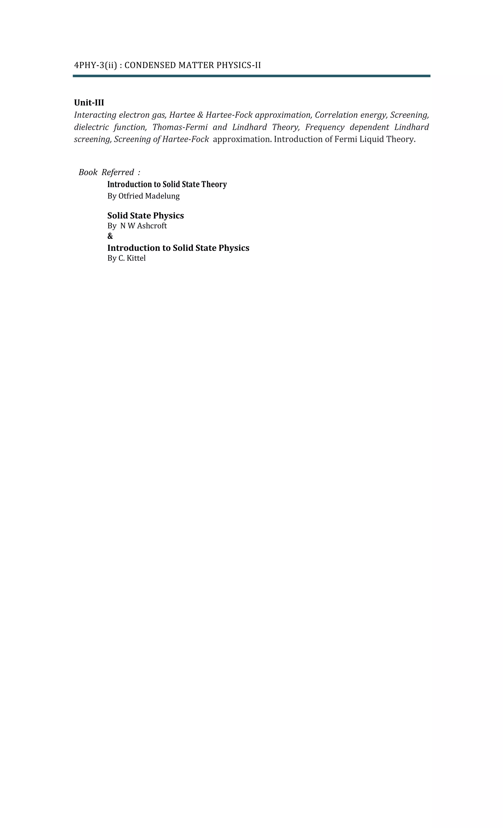
This is Hartree–Fock (HF) approximation. Now from variational calculation by putting
(11) into (9 ) leads to a set of Hartree–Fock equations:
2
2 2 2
*( ') ( ') *( ') ( ')
( ) ' ( ) ' ( ) ( )..........12
2 ' '
j j j i
i j i ij j
r r r r
V r e dr r e dr r E r
m r r r r
   
  
   
        
    
  
We may obtain a value for the total energy in the Hartree–Fock approximation and this
will
again contain a extra term is the exchange interaction. Thus energy eigen values in
Hartree-Fock approximation from (9) will be
2
2
*( ') ( ') *( ) ( )| | 1
'
| 2 '
*( ') ( ') *( ) ( )1
- '
2 '
j j i i
ii i j
j i i j
i j
r r r rH
E E e drdr
r r
r r r r
e drdr
r r
    
 
   


  


  
 
In the application of HF equations, it is usually assumed that the spatial part of the
wavefunction
is the same for spin-up and spin-down electrons, i.e., every orbital is doubly occupied,
and the
wavefunctions of the Slater determinant are spin singlets. This is so-called restricted
Hartree–Fock (HF) method, and can be reasonably used in many problems not
involving magnetism. In magnetic problems the HF equations are necessarily different.
Average energy per particle calculated from Hartree-Fock equation is better than
that from Hartree equation, but still binding is too weak. Major difficulty with Hartree-
Fock approximation is that the density of states at the Fermi level goes to zero.
The particle density of the other electrons felt by Hartree-Fock particle, looks like that
shown in Fig.
The concentration of the
electrons of like spin is
lowered in the
neighborhood of the
investigated electron. The
difference between the
Hartree and the Hartree-
Fock approximation is
that density of particles
for Hartree electron only
depends on position of
other electrons it is the same for
each position of the observed particle. But density of other electrons for Hartree-Fock
electrons depends on the position of the observed particle, i.e., on the position of the
particle for which we are actually solving the Hartree-Fock equation.
If the investigated electron i is at position r, then all other electrons of like spin are
displaced from position r. Due to the Pauli principle the electrons of like spin do not
move independently of each other, but their motion is correlated, because in its
neighborhood an electron displaces the other electrons. Another correlation due to the
Coulomb repulsion for all electrons, is included in an averaged way in Hartree as well as
in Hartree-Fock theory, so that the correlation resulting from the Coulomb repulsion is
missing in both theories. Hartree-Fock therefore contains a part of the correlation, the so-
called Pauli correlation.
3.4 Hartree Fock Theory of Free Electrons
In case of free electron gas the wave function is a plane wave of type,

5. 𝜓𝑖( 𝑟) =
𝑒 𝑖𝑘 𝑖.𝑟
√ 𝑉
𝑋 𝑠𝑝𝑖𝑛 𝑓𝑢𝑛𝑐𝑡𝑖𝑜𝑛
Because of free electrons the electron charge density is uniform all over the specimen.
Hence coulomb potential due to the electron is constant. Similarly ions are fixed at their
positions and having same charge density as that of electrons. Therefore potentials are
cancelled together and only the exchange term survives.
The Fourier transform of the term
𝑒2
|𝑟−𝑟′|
is given by,
𝑒2
|𝑟−𝑟′|
= 4𝜋𝑒2 1
𝑉
∑
1
𝑞2 𝑒−𝑖𝑞.(𝑟−𝑟′)
→ 4𝜋𝑒2
∫
𝑑𝑞
(2𝜋)3
1
𝑞2 𝑒−𝑖𝑞.(𝑟−𝑟′)
Using this value in exchange term in Hartree Fock equation and after simplifying we get,
𝐸( 𝑘) =
ħ2 𝑘2
2𝑚
−
2𝑒2
𝜋
𝑘 𝐹 𝐹(𝑥), where, 𝑥 =
𝑘
𝑘 𝐹
and 𝐹( 𝑥) =
1
2
+
1−𝑥2
4𝑥
𝑙𝑛 |
1+𝑥
1−𝑥
|
To compute the contribution of all electrons , say N, then total energy is obtained by
multiplying first term by 2 ( because of double spin), and dividing second term by 2 (
because when we are considering interaction electron with other electrons we are
counting each electron pair twice). That is
𝐸 = 2 ∑
ħ2 𝑘2
2𝑚
−
𝑒2 𝑘 𝐹
𝜋
∑ 𝐹(𝑥),
𝐸 = 2 ∑
ħ2 𝑘2
2𝑚
−
𝑒2 𝑘 𝐹
𝜋
∑
1
2
+
𝑘 𝐹
2
−𝑘2
2𝑘 𝐹 𝑘
𝑙𝑛 |
𝑘 𝐹+𝑘
𝑘 𝐹−𝑘
| since x = k/kF
By transforming summation to integration and simplifying we get,
𝐸 = 𝑁 [
3
5
𝐸 𝐹 −
3
4
𝑒2
𝑘 𝐹
𝜋
]
3.5 Correlation
The Hartree method is a good starting point for the discussion of electron-electron
interactions, but there are some shortcoming that we have assumed that at any particular
instant an electron does not care positions of others. The technical term for this is the
neglect of correlation. In reality electron motions are correlated for two reasons:
(a) Coulomb Correlation
Since electrons repel each other they will keep as far apart from each other as possible. If
we take the example of the hydrogen molecule from we can easily accept that at any
instant it would be highly unlikely for both electrons to be “on” the same atom. If we
know where electron one is then we can predict with good certainty where electron two
is, just on the basis of electrostatics. In the Hartree approximation we assume that any
particular electron does not know where other electron is at any moment, but only their
time-averaged positions. As a result the Hartree approximation allows electrons to
occasionally come very close to each other, Thus the Hartree approximation slightly
overestimates electron-electron repulsions.
(b) Exchange
Since electrons are not distinguishable and have half-integer spin, the wavefunction of an
N electron system must change sign on interchange of any two of its particles. Writing
each one electron wavefunction as the product of a “space function” and a “spin
function”, it can be shown that this fundamental requirement introduces a special form of
electron correlation that is electrons with parallel spins tend to avoid each other. Each
electron is said to carry around an exchange hole, a region in which other electrons with
the same spin are excluded.
The Exchange Energy
Because electrons are Fermions and obey Pauli’s principle, the total wave function of the
system must be antisymmetric (i.e. the wave function changes sign when two electrons
are interchanged). That prevent two electrons of the same spin to come close to each
other. This has nothing to do with Coulomb repulsion, it is a purely quantum mechanical
effect. To illustrate this, consider just a two electron wave function (where the electrons

6. have the same spin). Then by definition, antisymmetry of the wave function says that Ψ
(r1,r2)= -Ψ (r2,r1) where r1 and r2 are the positions of electrons 1 and 2, respectively. But
that means the wave function is identically zero when r1 = r2 (i.e., the electrons are on top
of each other). Since the probability is proportional to |Ψ|2
, and since the wave function
is a smooth function (i.e., it will be small even when r1 and r2 are similar), this is
equivalent to “keeping the electrons apart”. But because this quantum effect keeps the
electrons apart, we have overestimated the repulsive electron-electron interaction term in
the Coulomb energy above. The correction is called the exchange energy and it has the
value
𝐸𝑒𝑥𝑐ℎ𝑎𝑛𝑔𝑒 = −
0.916
𝑟
There is one other term, even when the electron gas is uniform. This arises from the fact
that even electrons of opposite spin avoid each other, because of the Coulomb force. This
is called a correlation energy. This is also a negative energy. It goes to a finite value as
the electron spacing parameter goes to zero (infinite density limit). And then there is an
energy that arises from the non-uniformity of the electron gas.
the correlation energy is usually defined as the difference between the exact and self-
consistent Hartree-Fock energies.
3.6 Thomas Fermi screening and Dielectric function
If the external potential V(r ) is applied to the electron gas then average electron
density no longer remain constant because electrons will get attracted towards maximum
of V(r ).
If we write spatially varying electron density as,
( ) ( )........1n r n n r 
Where n is the uniform density when V=0, then we can define induce charge density as,
( ).............2en r  
This induce charge density creates induced electrostatic potential δV, given by Poisson’s
equation as,
2
4 ..................3V  
Then total potential can be written as,
total total
............................4
consider this in Fourier space then V(k), V ( ), ( ), ( ) are the Fourier transform of V(r), V ( ),
( ), ( ) respectively. Then equation [4] become
totalV V V
k V k k r
V r r
V

 
 
 
2
( ) ( ) ( )............................5
Thus dielectric function is defined as,
( )
( ) ...............................6
( )
Since, k=i , equation [3] can be written as,
( ) 4 ( )
or,
total
total
k V k V k
V k
k
V k
k V k k


 
 



2
2
2
4
( )
k
Therefore, equation [5] become,
4
( ) ( )
k
( ) 4
, ( ) 1 ...............[7]
( ) k ( )
total
total total
V k
V k V k
V k
or k
V k V k



 


 
  

7. We now need to find that is induced in presence of ( ).
To compute the value of we assume the slowly varying V(r)
so that the system is remain in local equilibrium at every position of r.
T


totalV k
k total B
k B
(E -eV (k)- )/k
0 total
0 (E - )/k
hen in such case the probability of finding an electron with wave
vector k at postion r is given by Fermi function,
1
f(k,r)=
e 1
or, f(k,r)=f (k,μ+eV (k))
1
so, f (k,μ)=
e


T
 
3
0 total 03
3
0
3
3
2
03
2
, which is equilibrium distribution when V=0.
1
d
Thus (r)=-e f (k,μ+eV (k))-f (k,μ)
4
dfd k
or, δρ(r)=-e ( )
4π
d d k
or,δρ(r)=-e ( ) f ( )
4π
dn( )
or,δρ(r)=-e ( ) , where










T
total
total
total
k
eV r
d
V r k
d
V r
d
3
03
2
2
2
2
d k
n( )= f ( ) is the equilibrium density.
4π
dn( )
So also, δρ(k)=-e ( )
δρ(k) dn( )
or, =-e
( )
so, equation [6] become,
4 dn( )
( ) 1 e .........................[8]
k
This is Thomas F





 


 

total
total
k
V k
d
V k d
k
d
2
2 20
02
ermi equation for dilectric function and it can also be
written in the form as,
dn( )
( ) 1 , where 4 e
k

 

  
k
k k
d
To illustrate the significance of k0 , let us consider a point charge Q is placed in the metal
at a point r. Then external potential V is given by,
𝑉( 𝑟) =
𝑄
𝑟
𝑜𝑟 𝑉(𝑘) =
4𝜋𝑄
𝑘2
The potential I the metal will then be,
𝑉𝑡𝑜𝑡𝑎𝑙( 𝑘) =
𝑉( 𝑞)
𝜖( 𝑘)
=
4𝜋𝑄
𝑘2
2
0
2
1 ,
k

k
=
4𝜋𝑄
𝑘2 + 𝑘0
2
By inverting through Fourier transform we get,
𝑉𝑡𝑜𝑡𝑎𝑙( 𝑟) = ∫
𝑑3
𝑘
(2𝜋)3
𝑒 𝑖𝑘.𝑟
4𝜋𝑄
𝑘2 + 𝑘0
2 =
𝑄
𝑟
𝑒−𝑘0 𝑟
Thus the total potential is of Coulomb form times the exponential damping factor. Thus
potential reduces to negligible size at a distance greater than 1/k0. This form of potential
is known as screened Coulomb potential or Yukawa potential.
The Thomas Fermi method has the advantages that it is applicable even when a linear
relation between induced charge density and the potential does not hold. It has a
disadvantage that it is only for slowly varying external potentials.

8. 3.7 Lindhard Dielectric function
Consider a potential V(r) applied to the electron gas . To calculate the change in
electron density δn(r) we could calculate effect of V(r) on electron eigen sates.
Using Rayleigh-Schrodinger stationary perturbation theory for lowest order in V(r),
the eigen states become,
|𝜓 𝑘〉 = |𝑘〉 + ∑
|𝑘′〉⟨ 𝑘′| 𝑣(𝑟)| 𝑘⟩
𝐸𝑘 − 𝐸𝑘′
k'
Where |𝑘〉 is the unperturbed plane wave eigen state with energy E 𝑘=
ħ2 𝑘2
2𝑚
and
|𝜓 𝑘〉 is the new eigen function results from v(r).
The electron density as a function of position for wave function |𝜓 𝑘〉 is |〈 𝑟|𝜓 𝑘〉|2
SO chane in electron density due to perturbation is
|〈r|ψk〉|2
-|〈r|k〉|2
=〈ψk|r〉〈r|ψk〉 - 〈k|r〉〈r|k〉
=[〈r|k〉 + ∑
〈r|k'〉〈k'|v|k〉
𝐸 𝑘−𝐸 𝑘′
𝑘′ ] [〈k|r〉 + ∑
〈k'|r〉〈k|v|k'〉
𝐸 𝑘−𝐸 𝑘′
𝑘′ ] − 〈k|r〉〈r|k〉
To linear order in V above equation become
=∑ {
〈r|k〉〈k'|r〉〈k|v|k'〉
𝐸 𝑘−𝐸 𝑘′
+
〈k|r〉〈r|k'〉〈k'|v|k〉
𝐸 𝑘−𝐸 𝑘′
}𝑘′
Now we have , 〈r|k〉 =
𝑒 𝑖𝒌⃗⃗ .𝒓⃗
√ 𝑉
where V is the volume,
〈k|r〉 =
𝑒−𝑖𝒌⃗⃗ .𝒓⃗
√ 𝑉
and
〈k'|v|k〉 = ∫
1
𝑉
𝑒−𝑖𝒌′⃗⃗⃗⃗ .𝒓⃗
𝑣( 𝑟) 𝑒 𝑖𝒌⃗⃗ .𝒓⃗
𝑑3
𝑟
〈k'|v|k〉 =
1
𝑉
∫ 𝑒
−𝑖(𝒌′⃗⃗⃗⃗ −𝒌⃗⃗ ).𝒓⃗
𝑣(𝑟)𝑑3
𝑟
〈k'|v|k〉 =
1
𝑉
𝑣 𝒌′⃗⃗⃗⃗ −𝒌⃗⃗ is the Fourier transform of v(r).
So above equation become
〈k'|v|k〉 =
1
𝑉2 ∑ {
𝑒−𝑖(𝒌′⃗⃗⃗⃗ −𝒌⃗⃗ ).𝒓⃗
𝑣 𝒌⃗⃗ −𝒌′⃗⃗⃗⃗
𝐸 𝑘 − 𝐸 𝑘′
+
𝑒−𝑖(𝒌⃗⃗ −𝒌′⃗⃗⃗⃗ ).𝒓⃗
𝑣 𝒌′⃗⃗⃗⃗ −𝒌⃗⃗
𝐸 𝑘 − 𝐸 𝑘′
}
𝑘′
So total induced electron density will be obtained by summing over all
occupied states
δn(r) = 2 ∑ fk
k
1
𝑉2
∑
{
𝑒
−𝑖( 𝒌′⃗⃗⃗⃗
−𝒌⃗⃗ ).𝒓⃗⃗
𝑣 𝒌⃗⃗ −𝒌′⃗⃗⃗⃗
𝐸 𝑘 − 𝐸 𝑘′
+
𝑒−𝑖( 𝒌⃗⃗ −𝒌′⃗⃗⃗⃗ ).𝒓⃗⃗
𝑣 𝒌′⃗⃗⃗⃗ −𝒌⃗⃗
𝐸 𝑘 − 𝐸 𝑘′
}
𝑘′
where factor ‘2’ appears due to spin degeneracy and fk is the Fermi occupation
function fk =
1
𝑒
(𝐸 𝑘−𝜇) 𝑘 𝛽 𝑇⁄
+1
, where 𝑘 𝛽 is the Boltzmann constant and μ is chemical
potential.

9. Fourier transform to get δn(q)
δn(q) = ∫ 𝑒−𝑖𝒒⃗⃗ .𝒓⃗⃗
𝛿𝑛(𝑟)𝑑
3
𝑟
δn(q) =
1
𝑉2
2 ∑ 𝑓 𝑘 {
𝑉𝛿 𝑞,𝒌⃗⃗ −𝒌′⃗⃗⃗⃗ 𝑣 𝒌⃗⃗ −𝒌′⃗⃗⃗⃗
𝐸 𝑘 − 𝐸 𝑘′
+
𝑉𝛿 𝑞,𝒌′⃗⃗⃗⃗ −𝒌⃗⃗ 𝑣 𝒌′⃗⃗⃗⃗ −𝒌⃗⃗
𝐸 𝑘 − 𝐸 𝑘′
}
𝑘,𝑘′
now use 𝛿′
𝑠𝑡𝑜 𝑑𝑜 𝑠𝑢𝑚 𝑜𝑣𝑒𝑟 𝑘′ we get
δn(q) =
2
𝑉
∑ 𝑓 𝑘 {
𝑣 𝑞
𝐸 𝑘 − 𝐸 𝑘−𝑞
+
𝑣 𝑞
𝐸 𝑘 − 𝐸 𝑘+𝑞
}
𝑘
so,
δn(q)
𝑣 𝑞
=
2
𝑉
∑ 𝑓 𝑘 {
1
𝐸 𝑘−𝐸 𝑘−𝑞
+ 1
𝐸 𝑘−𝐸 𝑘+𝑞
}𝑘 now put 𝑘′
= 𝑘 − 𝑞
δn(q)
𝑣 𝑞
=
2
𝑉
∑
𝑓 𝑘+𝑞 − 𝑓 𝑘
𝐸 𝑘+𝑞 − 𝐸 𝑘
𝑘
δn(q)
𝑣 𝑞
= ∫
𝑓 𝑘+𝑞 − 𝑓 𝑘
𝐸 𝑘+𝑞 − 𝐸 𝑘
𝑑
3
𝑟
4𝜋3
For electrostatic potential 𝑣 𝑞 = −𝑒𝑉𝑞
𝑡𝑜𝑡𝑎𝑙
and 𝛿𝜌 = −𝑒𝛿𝑛, so
𝛿𝜌(𝑞)
𝑉𝑞
𝑡𝑜𝑡𝑎𝑙 =
−𝑒𝛿𝑛(𝑞)
𝑣(𝑞)
(−𝑒)⁄
𝛿𝜌(𝑞)
𝑉𝑞
𝑡𝑜𝑡𝑎𝑙 =
𝑒2
𝛿𝑛(𝑞)
𝑣(𝑞)
𝛿𝜌(𝑞)
𝑉𝑞
𝑡𝑜𝑡𝑎𝑙 = 𝑒2
∫
𝑓 𝑘+𝑞−𝑓 𝑘
𝐸 𝑘+𝑞−𝐸 𝑘
𝑑3 𝑟
4𝜋3
………………..[1]
For small q 𝑓𝑘+𝑞 − 𝑓𝑘 ≈
𝜕𝑓
𝜕𝑞
. 𝑞
And 𝐸 𝑘+𝑞 − 𝐸 𝑘 ≈
𝜕𝐸
𝜕𝑞
. 𝑞
Therefore [1] become
𝛿𝜌(𝑞)
𝑉𝑞
𝑡𝑜𝑡𝑎𝑙
= 𝑒2
∫
𝜕𝑓
𝜕𝐸
𝑑3
𝑟
4𝜋3
= 𝑒2
∫
𝜕𝑓
𝜕𝐸
𝑑𝐸 𝑔(𝐸)
As 𝑇 → 0,
𝜕𝑓
𝜕𝐸
→ −𝛿(𝐸 − 𝐸 𝐹)
So we get,
𝛿𝜌(𝑞)
𝑉𝑞
𝑡𝑜𝑡𝑎𝑙 = −𝑒2
𝑔(𝐸 𝐹)
As dielectric function , 𝜖( 𝑞) = 1 −
4𝜋
𝑞2
𝛿𝜌(𝑞)
𝑉𝑞
𝑡𝑜𝑡𝑎𝑙 , we get
𝜖( 𝑞) = 1 +
4𝜋
𝑞2
𝑒2
𝑔(𝐸 𝐹) ……………………………..2
Thus it is seen that Lindhard dielectric function is same as Thomas –Fermi function.

10. Friedel Oscillations (Linhard dielectric function at higher ‘q’)
We have fron equation [2],
𝜖( 𝑞) = 1 +
4𝜋
𝑞2
𝑒2
𝑔(𝐸 𝐹)
𝜖( 𝑞) = 1 +
4𝜋
𝑞2
𝑒2 ∑
𝑓 𝑘−𝑓 𝑘+𝑞
𝐸 𝑘+𝑞−𝐸 𝑘
𝑘 ……………….3
Since
𝐸 𝑘 =
ħ2 𝑘2
2𝑚
we get,
𝐸 𝑘+𝑞 − 𝐸 𝑘 =
ħ2( 𝑘 + 𝑞)2
2𝑚
−
ħ2
𝑘2
2𝑚
=
ħ2
𝑞2
2𝑚
+
2ħ2
𝐤. 𝐪
2𝑚
=
( 𝑞2
+ 2𝐤. 𝐪)ħ2
2𝑚
Therefore equation [3] become
𝜖( 𝑞) = 1 +
4𝜋
𝑞2
𝑒2 2𝑚
ħ2 ∫
𝑑3 𝑘
8𝜋3𝑅
1
(𝑞2+2𝐤.𝐪)
× 2 × 2
Here R represent the region of k-
space where k if full and k+q is
empty First factor ‘2’ appears in
above equation because of spin up
and spin down similarly second ‘2’
appears when Fermi sphere k+q if
full and k is empty.
If q increases then region R is also increases. We can show it graphically as follow,
The integral
𝜖( 𝑞) = 1 +
4𝜋
𝑞2
𝑒2
2𝑚
ħ2
∫
𝑑3
𝑘
8𝜋3
𝑅
1
( 𝑞2 + 2𝐤. 𝐪)
× 2 × 2
By solving the integral explicitly we get,
𝜖( 𝑞) = 1 +
4𝜋𝑒2
𝑞2
𝑞( 𝐸 𝐹) [
1
2
+
1 − 𝑥2
4𝑥
𝑙𝑛 |
1 + 𝑥
1 − 𝑥
|]
Where 𝑥 =
𝑞
2𝑘 𝐹
As 𝑥 → 0, 𝑡ℎ𝑒 𝑏𝑟𝑎𝑐𝑘𝑒𝑡 𝑡𝑒𝑟𝑚 =
1 𝑎𝑛𝑑 𝑤𝑒 𝑔𝑒𝑡 𝑏𝑎𝑐𝑘 𝑇ℎ𝑜𝑚𝑎𝑠 𝐹𝑒𝑟𝑚𝑖 𝑑𝑖𝑒𝑙𝑒𝑐𝑡𝑟𝑖𝑐 𝑓𝑢𝑛𝑐𝑡𝑖𝑜𝑛
𝑎𝑛𝑑 𝑎𝑡 𝑥 = 1 𝑡ℎ𝑎𝑡 𝑖𝑠 𝑓𝑜𝑟 𝑞 = 2𝑘 𝐹, 𝑡ℎ𝑒𝑛 𝜖( 𝑞) ~
1
𝑟3
cos(2 𝑘 𝐹 𝑟)
So
𝜖( 𝑞) 𝑜𝑟 𝑖𝑛𝑑𝑢𝑐𝑒𝑑 𝑐ℎ𝑒𝑟𝑔𝑒 𝑑𝑒𝑛𝑠𝑖𝑡𝑦 𝑑𝑒𝑐𝑎𝑦𝑠 𝑚𝑜𝑟𝑒 𝑠𝑙𝑜𝑤𝑙𝑦 𝑎𝑛𝑑 𝑜𝑠𝑐𝑖𝑙𝑙𝑎𝑡𝑒𝑠 𝑎𝑠𝑎 𝑐𝑜𝑠𝑖𝑔𝑛 𝑓𝑢𝑛𝑐𝑡𝑖𝑜𝑛.
This is known as Friedel oscillations.