Tesi

Alma Mater Studiorum · University of Bologna
FACULTY OF MATHEMATICAL, PHYSICAL AND NATURAL SCIENCES
Master degree in Mathematics
Interactions between overlapped wells:
study of the resonances
Degree thesis in Quantum Mathematical Physics
Advisor:
Prof. A. G. Martinez
Presented by
Jacopo Lanzoni
Key words: Born-Oppenheimer approximation; quantum resonances;
semiclassical analysis; microlocal interactions; pluriatomic molecules.
I session
Academic Year 2009-2010

To my parents
Iader and Loriana

Contents
1 Introduction: Born-Oppenheimer approximation 5
2 The diatomic case 9
3 The multidimensional model 15
4 The reduction to a self-adjoint problem 19
5 Interaction estimate 25
3

Chapter 1
Introduction: Born-Oppenheimer
approximation
In quantum physics, time evolution of a molecule is described by the solution φ of
the initial value problem for the Schrödinger equation
i∂tφ = Hφ
φ|t=0 = φ0
(1.1)
where φ0 is the initial state of the molecule and H the molecular Hamiltonian, which
contains the interactions between the particles constituting the molecule - electrons and
nuclei - and the potentials of the eventual electric field where the molecule is submerged.
In the case of a free molecule, i.e. not submerged in any field, a first approach to
study the system (1.1) consists in neglecting the motion of the centre of mass and in
considering only bounded initial state, that is the initial states which are eigenfunctions
of the Hamiltonian. More precisely, one can divide the Hamiltonian in
H = HCM + HRel,
with the operators HCM , which is the kinetic energy of the centre of mass, and HRel,
which is the relative motion of electrons and nuclei, which commutes each other. Of
consequences, quantum evolution factorizes in
e−itH
= e−itHCM
e−itHRel
,
where free evolution e−itHCM
of the centre of mass can be calculated explicitly as HCM has
constant coefficients, while the relative motion e−itHRel contains the interactions which
makes the solution of the problem more difficult. Then taking φ0 of the form
φ0 = α0 ⊗ ψj, (1.2)
5

with α0 depending only by the position of the centre of mass and ψj eigenfunction of
HRel relative to the eigenvalue Ej, the solution of (1.1) is given by
φ(t) = e−itEj
(e−itHCM
α0) ⊗ ψj.
In this case the real problem is to know well enough the eigenvalues of HRel to be able
of build an initial state of the form (1.2).
In 1927 Max Born and Robert Oppenheimer (see [2]) proposed a method to make
such an approximation of eigenvalues and eigenfunctions of HRel. The method is based
on the fact that nuclei are much more heavier than electrons, so their motion is slower
and makes electrons adapt almost instantly. Consequently, the motion of electrons is not
really perceived by nuclei, except that for an electric field created by their total potential
energy, that becomes function of nuclei position. In this way, molecules evolution reduces
to nuclei evolution in a effective electrical potential created by electrons. Such a reduction
permits in a second time to use semiclassical tools in order to find eigen-elements of final
effective Hamiltonian.
Let M be the nucleus mass and m the electron one: let’s put for simplicity m = 1
and define the parameter
h :=
1
M
.
Given a molecule made of n atoms and submerged in a extern electromagnetic field, the
Hamiltonian operator is
H = −
1
2M
∆x + Q(x), on H = (L2
(R3
))⊗n
where the self-adjoint operator (∆x, (H2
(R3
))⊗n
) represents the kinetic energy of the
nuclei of mass M, while the operator Q(x) represents the electronic Hamiltonian with
interactions and eventual extern fields. Let us assume that Q(x), which sends the posi-
tion x of the nuclei the position y of electrons, admit an isolated eigenvalue λ(x) with
eigenfunction ψ(x, y),
Q(x)ψ(x, y) = λ(x)ψ(x, y), ψ(x, ·) = 1;
we look for φ of the form
φ(x, y) = f(x)ψ(x, y),
where f(x) is a coherent state in the variable x. So far, the eigenvalue equation Hφ = Eφ
can be written as
−
1
2M
∆x[f(x)ψ(x, y)] + Q(x)f(x)ψ(x, y) = Ef(x)ψ(x, y),
−
1
2M
[∆xf(x)ψ(x, y)+ xf(x) xψ(x, y)+f(x)∆xψ(x, y)]+f(x)Q(x)ψ(x, y) = Ef(x)ψ(x, y),
6

−
1
2
h2
[∆xf(x)ψ(x, y)+ xf(x) xψ(x, y)+f(x)∆xψ(x, y)]+f(x)λ(x)ψ(x, y) = Ef(x)ψ(x, y),
−
1
2
h2
∆xf(x) + λ(x)f(x) − Ef(x) ψ(x, y)−h2
[ xf(x) xψ(x, y) + f(x)∆xψ(x, y)] = 0.
The theory of Born-Oppenheimer consists in neglecting at this point the f ψ + f∆ψ
term, and in approximating the previous equation with the simpler
−
1
2
h2
∆x − λ(x) − E f(x) = 0.
To better understand the nature of such an approximation, we are going to talk about
’order’. A semiclassical differential operator P(x, Dx; h) of degree m can be written in
the form P(x, hDx; h) as
P(x, hDx; h) =
|α|≤m
aα(x)(hDx)α
+
K
k=1
hk
|α|≤m
ak,α(x)(hDx)α
, (1.3)
and we use to say it has order K. So far, we say a semiclassical differential operator
P(x, Dx; h) of degree m has order zero if it can be written in the form P(x, hDx; h) as
P(x, hDx; h) =
|α|≤m
aα(x)(hDx)α
.
As in quantum physics such operators are tipically applied to functions of the form
f(x; h) = eiφ(x)/h
(WKB approximation, cfr. [8]), we get
hDxf(x; h) = h
1
i
∂xeiφ(x)/h
= h
1
i
eiφ(x)/h i
h
∂xφ(x) = ∂xφ(x) · f(x; h),
that is, the operator hDx reduces to multiplication with the gradient of the phase. Now
it is clear why, for small values of h, the second term in the approximation (1.3) is
‘neglectable’ with respect to the first one.
Writing
φ0(x, y) = f(x)ψ(x, y) +
k≥1
hk
φ0,k(x, y) = f(x)ψ(x, y) + O(h),
for φ0,k opportunely chosen, then we deduce
φt(x, y) = ft(x)ψ(x, y) +
k≥1
hφ
t,k(x, y),
where ft and φt,k can be explicitly computed through the classic flux of effective Hamil-
tonian Heff(x, ξ) := Kn(ξ) + λ(x) (see definition 3.1).
7

More generally, we can define the electronic levels λ1(x) ≤ λ2(x) ≤ · · · ≤ λn(x)
as the eigenvalues of Q(x); so far, the Born-Oppenheimer approximation consists in
substituting the operator Q(x) with a matrix operator of the form
Q (x, M) :=





λ1(x) 0 . . . 0
0 λ2(x)
...
...
... 0
0 . . . 0 λn(x)





+
1
√
M
R x,
1
√
M
Dx ,
where R is a square matrix of dimension n whose entries are pseudodifferential opera-
tors. With Born-Oppenheimer approximation we reduce in studying the ’approximated’
Schrödinger equation ih∂tφ = P(h)φ, with
P(h) = −
h2
2
∆xIn + Q (x) + hR(x, hDx),
where In is the identity matrix of dimension n.
In this work I will deal with this operator in the diatomic case (that is with n = 2),
with particular attention to the resonances generated by ’overlapped wells’ potentials.
8

Chapter 2
The diatomic case
The chapter is devoted to the exposition of the known results in the case of a single
diatomic molecule (n = 2), following the work [4] by Grecchi, Kovarik, Martinez, Sac-
chetti and Sordoni. In brief, if x1, x2 ∈ R3
are the coordinates of the two atoms of the
molecule, we fix the position of one of them as the origin of the cartesian system and
we indicate the coordinates of the second as R = x2 − x1, R := |R|, and the position
of the electron with r. So far, for rotation invariant potentials, we get a operator P
which is still invariant. Passing to polar coordinates and fixing the value of the angular
momentum, we reduce to a one-dimensional problem.
Figure 2.1: The diatomic case.
Let us consider the time-independent Schröringer equation with Hamiltonian operator
of the form
H = −h2
∆R +
1
R
+ He (2.1)
9

where h << 1 and He is the electronic Hamiltonian, formally defined on L2
(R3
r) as
He := He(R) = −∆r −
1
|r − 1
2
R|
−
1
|r + 1
2
R|
+ V, (2.2)
where V is the extern potential. The operator (2.1) acts on the Hilbert space
K = L2
(R3
R; L2
(R3
r)).
The analysis of such a three-body problem is difficult, and we need to introduce
further hypothesis. Let us assume the potential V depends only on the component of
the vector r along the direction R. So far, it is possible to introduce a rotation which
commute with H, and so we find the spectrum of the electronic Hamiltonian He(R)
depends only on R := |R|.
Now, indicating with LR and Lr the angular moment with respect to R and to r, we
see that [H, LR + Lr] = 0. In the following, we will particularly interested in the eigenval-
ues and in the resonances of the restrictions of H to the invariant subspace Ker(LR + Lr).
This corresponds in some way to fix to zero the rotational energy of the molecule. Af-
ter Born-Oppenheimer reduction to an effective Hamiltonian P = P(R, hDR), this is
equivalent to the study of the restriction of P to Ker(LR).
For every fixed R ∈ Rn
, we indicate with Sp(He(R)) the spectrum of the electronic
Hamiltonian operator He(R) defined on the Hilbert space L2
(R3
r), which depends only
on R. Let us assume such a spectrum contain at least two eigenvalues, whose the first
two λ1(R) and λ2(R)
• are non-degenerated;
• olomorphically extends in a sharp complex neighborhood Γδ of the real line;
• are such that
lim
Γδ R→∞
λ1(R) =: λ∞
1 < λ∞
2 := lim
Γδ R→∞
λ2(R).
Moreover, let us assume the first two eigenvalues and the rest of the spectrum are dis-
tinguished.
Let us indicate the effective potential associated to the jth
eigenvalue with
Vj(R) =
1
R
+ λj(R).
Let us suppose also the effective potential is such that
• is an analytic function with respect to R;
• when R → 0+, Vj(R) → +∞;
10

• the effective potential V1 has the shape of a well, with non-degenerate minimum
m1 in a point Rm
1 and the barrier non-degenrate maximum M1 in a point RM
1 .
Moreover, V1 doesn’t admit other critical point in the domain V −1
1 ([m1, M1]). The
effective potential V2 has the shape of a well too, with local minimum m2 in a point
Rm
2 .
In polar coordinates the Hamiltonian (2.1) has the form
H = −h2 ∂2
∂R2
+
2
R
∂
∂R
− h2 1
R2
1
sin θ
∂
∂θ
sin θ
∂
∂θ
+
1
sin2
θ
∂2
∂θ2
+
1
R
+ He(R) (2.3)
The operator −h2
R−2
[(sin θ)−1
∂θ sin θ∂θ + (sin θ)−2
∂2
θ ] has eigenvalues h2
R−2
l(l + 1) for
every l ∈ N. Then a rotation exists which gives to the operator H the form
H = −h2 ∂2
∂R2
+
2
R
∂
∂R
+ h2 l(l + 1)
R2
+
1
R
+ He(R) su L2
(R+, R2
dR; L2
(R3
r)).
Finally, taking l = 0, that is considering the restriction of H to Ker(LR), and changing
the variable ψ(R, r) → Rψ(R, r), the Hamiltonian H takes the form
H0 = −h2 ∂2
∂R2
+
1
R
+ He(R) su L2
(R+, dR; L2
(R3
r)),
with Dirichlet boundary condition at R = 0.
With Born-Oppenheimer approximation we can transform the previous Hamiltonian
in the reduct operator
Pj = −h2 d2
dR2
+ Vj(R) on L2
(R+, dR), (2.4)
for j = 1, 2 and with boundary condition at R = 0. Then, it follows that for 0 < h << 1
and for a small extern field, the discrete spectrum of Pj in the interval [mj, E∞
j ) is
not empty. In the case of non-degenerate minima, we know the distance between the
eigenvalues is of order h with h → 0.
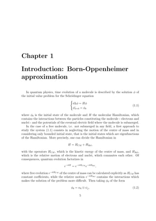
Let us formally define the differential operator
P = −h2
∆R
1 0
0 1
+
V1(R) 0
0 V2(R)
+ h2 0 a(R)
a0(R) 0
DR
with a0 ∈ C∞
b .
For such an operator one knows some important results, but before stating them we
need to give the definition of analytic distorsion, both of a function and of an operator.
11

Definizione 2.1. Let be µ << 1 and s ∈ C∞
(R), 0 ≤ s ≤ 1 with s(x) = 0 on a compact
neighbouroohd of the origin, s(x) = 1 for |x| >> 1. Let us set
Iµ : Rn
R −→ (1+µs(R))R ∈ Rn
, Jµ : R6
(R, r) −→ 1 + µs
R
R
, r r ∈ Rn
,
and define the analytic distorsione of the test function φ with the formula
Sµφ(R, r) := |J(R, r)| φ(Iµ(R), Jµ(R, r)),
where J(R, r) is the Jacobian of the transformation Fµ given by Fµ : R6
−→ R6
,
Fµ(R, r) := (Iµ(R), Jµ(R, r)). Let us set also φµ : R+ −→ R+, φµ(R) := R(1 + µs(R)).
We define the analytic distorsion of an operator A as
Aµ := SµAS−1
µ .
We are now able to understand the two main results of the work [4] of Grecchi,
Kovarik, Martinez, Sacchetti and Sordoni. In the following, Pµ and PD indicates the
analytic distorsion of P and its Dirichlet realization on the interval [0, RM
1 ], with RM
1
point of maximum for V1, respectively.
Teorema 2.1. Let be 0 < α << 1 and J ⊂ (0, 1], with 0 ∈ J , such that there exists a
function a(h) > 0 defined for h ∈ J for which
∀ > 0, ∃ C > 0 : a(h) ≥
1
C
e− /h
per h ∈ J , 0 < h << 1;
then it holds
Sp(PD) ∩ [m2 + α − 2a(h), m2 + α + 2a(h)] = ∅.
Let us set
Ω(h) := z ∈ C; dist(Re z, [m1, m2 + α]) < a(h), |Im z| < Ch ln
1
h
,
with C >> 1. Then there exist δ0 > 0 and a bijection
b : Sp(PD) ∩ [m1, m2 + α] −→ Sp(Pµ) ∩ Ω(h),
such that
b(λ) − λ = O(e−δ0/h
),
uniformly for h ∈ J .
Proof. See the proof of proposition 4.2 in [4].
12

So the resonances of P in Ω(h) coincide, but for an exponentially small error term,
to the eigenvalues of PD in the interval [m1, m2 + α]. But we can state even more.
Teorema 2.2. For 0 < h << 1 the resonances of P with real part in [m1, m2 + α]
and imaginary part << |h ln h| coincide, but for a O(h2
)-small error term, with the
eigenvalues of the Dirichlet realizations of P1,0 and P2,0 on (0, RM
1 ),
Proof. See the pages before theorem 4.8 in [4].
13

Chapter 3
The multidimensional model
In this chapter we begin the original part of the thesis, describing the model with
overlapped wells potential which we will work on.
Before describing the overlapped wells potential, we give some preliminary notions.
Let be f = f(x, ξ) ∈ C∞
(R2n
), defined from Hf to df(x, ξ), u = σ(u, Hf (x, ξ)) for every
u ∈ Tx,ξR2n
with σ the canonical symplectic form, i.e. the canonical transformation
(x, ξ) → exp tHf (x, ξ) is the Hamiltonian flux associated to f.
Definizione 3.1. A point (x, ξ) ∈ R2n
is said to be non-trapping for f if
lim
|t|→∞
|exp tHf (x, ξ)| = ∞.
A subset Ω ⊂ R2n
is said to be non-trapping for f if every (x, ξ) ∈ R2n
is non-trapping
for f. We also say a set I ⊂ R is non-trapping for f if f−1
(I) is non-trapping for f.
Let now V1, V2 ∈ C∞
(Rn
, R) be such that:
• V2 > V1;
• there exists m2 := minx∈Rn V2(x);
• there exist l2 := limx→∞ V2(x) and l1 := limx→∞ V1(x), and l1 < m2 < l2;
• the set {V1 < m2} is the disjoint union of a connected bounded set U, called ‘well’,
and of an unbounded open set M, called ‘sea’:
{V1 < m2} = U ∪ M;
• on M, m2 is non-trapping for the energy function of the first electronic level, i.e.
the set (M×Rn
)∩{ξ2
+V1 = m2} is non-trapping for the Hamiltonian ξ2
+V1(R).
15

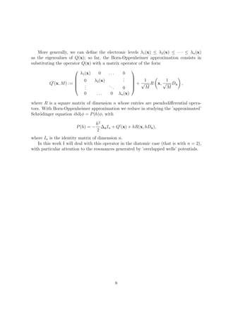
Figure 3.1: Section of two possible potential V1 and V2, seen by high.
Let us now consider the matrix operator P on the Hilbert space H = L2
(Rn
, C) ⊗
L2
(Rn
, C) with
P = h2
D2
xI2 +
0 α(x) · h2
Dx
h2
Dx · α(x) 0
+
V1(x) 0
0 V2(x)
,
where α ∈ C∞
b (Rn
, Cn
), |α(x)| −→ 0 if |x| → ∞, and let us look for the solutions of the
eigenvalue equation
Pφ(x) = λφ(x), λ ∈ C, φ(x) =
φ1(x)
φ2(x)
. (3.1)
If we set Pj = h2
D2
x + Vj(x) for j = 1, 2, the equation (3.1) becomes
(P1 − λ)φ1(x) = −hα(x)Dxφ2(x), (P2 − λ)φ2(x) = −hα(x)Dxφ1(x).
For Weyl’s theorem, which states a relatively compact perturbation leaves essential
spectrum invariant of a self-adjoint operator, we have
Spess(P) = Spess(h2
D2
xI2 + V (x)),
and so
Spess(P) = Spess(h2
D2
x + V1(x)) ∪ Spess(h2
D2
x + V2(x)).
Using again Weyl’s theorem, we get
Spess(P) = [l1, +∞) ∪ [l2, +∞) = [l1, +∞).
Now we want to study the resonances λ ∈ [m2, m2 + α] of operator P. In order to
distort it, we have to assume that:
16

Figure 3.2: Sector Σ in the complex plane with C = 4.
• V1, V2 and α are holomorphic in a sector Σ := {|Rex| ≥ C, |Imx| < 1/C|Rex|};
• for j = 1, 2 the following conditions holds:
lim
|x|→∞, x∈Σ
Vj(x) = lj, lim
|x|→∞, x∈Σ
α(x) = 0;
In questo modo possiamo deﬁnire Pµ il cui spettro essenziale `e
Spess(Pµ) = e−iµ
[l1; +∞) ∪ e−iµ
[l2; +∞).
Figure 3.3: Complex plane with essential spectrum of the distorted operator Pµ where
µ = 1, l1 = 3 and l2 = 6.
17

Chapter 4
The reduction to a self-adjoint
problem
In this chapter we show the eigenvalues of Pµ with real part in [m2 − α, m2 + α]
coincides, but for an exponentially small error term, with the eigenvalues of the Dirichlet
realization of PD of P on an open set B ⊂ Rn
which is in an island and which conains
the well. For λ < m2 − α, the problem can be reduced to a scalar one, as P2 ≥ m2 as
operator.
Proposizione 4.1. Let be 0 < α << 1, and J ⊂ (0, 1], with 0 ∈ J , such that there
exists a function a(h) > 0 deﬁned for h ∈ J and such that
∀ > 0, a(h) ≥
1
C
e− /h
∀ h << 1,
and that
Sp(PD)∩[m1 +α−2a(h), m1 +α+2a(h)] = ∅ = Sp(PD)∩[m2 +α−2a(h), m2 +α+2a(h)].
Setting
Ω(h) := z ∈ C; dist(Re[z], [m2 − α, m2 + α]) < a(h), Im[z] < Ch ln
1
h
with C >> 1, then there exist δ0 > 0 and a bijection
b : Sp(PD) ∩ [m2 − α, m2 + α] −→ Sp(Pµ) ∩ Ω(h)
such that
b(λ) − λ = O(e−δ0/h
),
uniformly for h ∈ J .
19

Proof. Let us first fill the hole of the well: we consider an open set B ⊂ Rn
which is in
the island and which contains the well, and we fix a function F = F(x) ∈ C∞
0 (B; R+)
such that
inf
x∈B
(V1 + F)(x) > m2 + α.
For j = 1, 2, we then indicate with pj,µ = pj,µ(x, x∗
) the principal symbol of the distorted
operator Pj,µ, symbol which we suppose to be analytic.
Now, as the energetic interval [m2 − α, m2 + α] is non-trapping for the operator
P1,µ + F(x), following section 4 of [10] we can consider a real function f0 = f0(x, x∗
) ∈
C∞
0 ((Rn
SuppF) × Rn
) such that on the set
(x, x∗
) ∈ R6
; F(x) + Re[p1(x, x∗
)] ∈ [m2 − α − δ; m2 + α + δ] , with 0 < δ << 1,
one has
−Im p1,µ x − h ln
1
h
( xf0 + i x∗ f0); x∗
− h ln
1
h
( xf0 − i x∗ f0) ≥
1
δ
h ln
1
h
.
Consequently, if z ∈ C is such that dist(z, [m2 − α, m2 + α]) = O(|h ln h|), then the
operator P1µ + F(x) − z is invertible on L2
(Rn
) with inverse such that it satisfy
h−f0
T(P1,µ + F(x) − z)−1
u L2(R6) ≤ C|h ln h|−1
h−f0
Tu L2(R6), (4.1)
where C > 0 is a constant and
T : L2
(Rn
) −→ L2
(R6
), Tu(x, x∗
) :=
1
2πh
ei
(x−x )x∗
h
−
x−x 2
2h u(x )dx
is the F.B.I. transform, i.e. the transform of Fourier-Bros-Iagolnitzer (cfr. chapter 3 in
[8]). Equivalently, for v = (P1,µ + F(x) − z)−1
u with u varying in L2
we have
h−f0
Tv L2(R6) ≤ C|h ln h|−1
h−f0
T(P1,µ + F(x) − z)v L2(R6),
and for density we can extend such estimate to every v ∈ (H2
∩ H1
0 )(Rn
). Now, the
inequality (4.1) holds for v = (P1,µ + F(x) − z)−1
u with u varying L2
. This means the
operator (P1,µ +F(z)−z)−1
has norm O(|h ln h|−1
) if we consider it on the space L2
(Rn
)
with norm
u H := h−f0
Tu L2(R6).
On the other hand, for construction, the operator P2,µ + F(x) has real part bigger
than m2 + α, and so, if Re[z] ≤ m2 + α, we see the operator (P2,µ + F(x) − z)−1
has
uniformly bounded norm on H.
Now, we choose due functions χ1, χ2 ∈ C∞
0 (B; [0, 1]) such that χ1 = 1 in a neighbor-
hood of Supp(χ2) and χ2 = 1 in a neighborhood of Supp(F). Setting
Qµ := Pµ + F(x); Rµ(z) := χ1(PD − z)−1
χ2 + (Qµ − z)−1
(1 − χ2), (4.2)
20

we see that, if dist(z, Sp(PD)) ≥ a(h), then
(Pµ − z)Rµ(z) = I + Kµ(z)
where
Kµ(z)
def
= [PD, χ1](PD − z)−1
χ2 − F(x)(Qµ − z)−1
(1 − χ2)
because
(Pµ − z)Rµ(z) = (Pµ − z)χ1(PD − z)−1
χ2 + (Pµ − z)(Qµ − z)−1
(1 − χ2) =
= (PD − z)χ1(PD − z)−1
χ2 + (Qµ − F(x) − z)(Qµ − z)−1
(1 − χ2) =
= (PD − z)χ1(PD − z)−1
χ2 + (Qµ − z)(Qµ − z)−1
(1 − χ2) − F(x)(Qµ − z)−1
(1 − χ2) =
= [PD, χ1](PD −z)−1
χ2 +χ1(PD −z)(PD −z)−1
χ2 +(I −χ2)−F(x)(Qµ −z)−1
(1−χ2) =
= [PD, χ1](PD − z)−1
χ2 + χ1χ2 + (I − χ2) − F(x)(Qµ − z)−1
(1 − χ2) =
= [PD, χ1](PD − z)−1
χ2 + χ2 + (I − χ2) − F(x)(Qµ − z)−1
(1 − χ2) =
= I + [PD, χ1](PD − z)−1
χ2 − F(x)(Qµ − z)−1
(1 − χ2).
Now, [PD, χ1] is a differential operator whose coefficients have supports in that of the
gradient of χ1; this is disjoint by the support of χ2, so the first term of Kµ(z) is zero.
Also F(x) and 1 − χ2 have supports which are disjoint and separted by a region where
inf V1 > m2 + α. So we can apply Agmon’s estimate
Re eφ/h
(−h2
∆ + V1 − E)u, eφ/h
u = h (eφ/h
) 2
+ (V1 − E − | φ|2
)eφ/h
u, eφ/h
u ,
(4.3)
to get (cfr. [6]) the estimate
Kµ(z) H = O(e−2δ/h
).
For such values of z and for sufficiently small value of h, we have
(Pµ − z)−1
= Rµ(z)
j≥0
(−Kµ(z))j
, (4.4)
and as for every such z there exists a certain constant C > 0 such that Rµ(z) H =
O(1/a(h)), we deduce if γ is a closed oriented simple path around Sp(PD)∩[m2−α, m2+α]
such that dist(γ, Sp(PD)) ≥ a(h) and dist(γ, [m2 − α, m2 + α]) << |h ln h|, then
Πµ :=
1
2πi γ
(z − Pµ)−1
dz = −
1
2πi γ
Rµ(z)dz −
1
2πi j≥1 γ
Rµ(z)(−Kµ(z))j
dz =
=
1
2πi γ
χ1(z − PD)−1
χ2dz −
1
2πi γ
(Qµ − z)−1
(1 − χ2)dz + O(e−2δ/h
)
21

=
1
2πi γ
χ1(z − PD)−1
χ2dz + O(e−2δ/h
) = χ1ΠDχ2 + O(e−2δ/h
). (4.5)
with (Qµ − z)−1
holomorphic in the interior of γ and
ΠD :=
1
2πi γ
(z − PD)−1
dz.
So,
Πµ − χ1ΠDχ2 << 1
from which it follow that Πµ and χ1ΠDχ2 have the same rank.
Since Πµ is the spectral projector of Pµ associated to Ω(h), the corresponding res-
onances of P are nothing but the eigenvalues of PµΠµ restricted to the values of Πµ.
Moreover, if we set {µ1, . . . , µm} := Sp(PD) ∩ [m1, m2 + α] and let {φ1, . . . , φm} be
an orthonormal basis of Ker(PD − µj), then for Agmon estimates (4.3) we see from
(4.5) that the functions Πµχ1φj, j = 1, . . . , m, are a basis of Im(Πµ), and the matrix of
Pµ|Im(Πµ) with respect to this basis has the form diag(µ1, . . . , µm)+O(e−δ/h
). The result
comes from m = O(h−n
) and from the following argument on the eigenvalues of matrices:
Lemma 4.2. Let M and N be two matrices of dimension d = O(h−n
) such that:
i. M = diag(µ1, . . . , µd);
ii. M + N = O(1);
iii. ∃ c, δ > 0 : M − N ≤ ce−δ/h
.
Then there exist δ > 0 and a bijection
β : Sp(M) −→ Sp(N)
such that
|λ − β(λ)| = O(e−δ /h
)
Proof. First of all we show that Sp(M)⊂ B(µj; 2ce−δ/h
) proving
C
d
j=1
B(µj; 2ce−δ/h
) ⊂ ρ(M).
Indeed, if |z − µj| ≥ 2ce−δ/h
then, set R := M − N, we have N − z = M − z + R =
(I + R(M − z)−1
)(M − z) is invertible because
R(M − z)−1
≤
1
2ce−δ/h
ce−δ/h
=
1
2
.
22

We then deﬁne for t ∈ [0, 1] the t-continuous deformation
Tt := (1 − t)N + tM
of the matrix T0 = M in the matrix T1 = N. We know that in these cases the eigenvalues
λj(t), j = 1, . . . , d, of Tt are such that for every j = 1, . . . , d:
• λj(0) = µj;
• λj(t) depend continuously on the parameter t ∈ [0, 1];
• λj(1) belong to the union of the balls B(µj; 2ce−δ/h
).
So, it holds that |Im(λj(t))| ≤ 2ce−δ/h
for every j = 1, . . . , d and for every t ∈ [0, T], and
that the union of the real parts of the balls B(µj; 2ce−δ/h
) is the disjoint union of the
intervals Ik(h)
d
j=1
Re(B(µj; 2ce−δ/h
)) =
d
k=1
Ik(h)
with Ik(h) such that
|Ik(h)| ≤
d
j=1
|λj(1) − µj| =
d
j=1
|λj(1) − λj(0)| ≤
d
j=1
2ce−δ/h
= d2ce−δ/h
= 2ch−n
e−δ/h
.
For every j = 1, . . . , d and for every t ∈ [0, 1] Re(λj(t)) and µj = Reλj(0) belong
for continuity to the same interval Ik(h), so |µj − Re(λj(t))| ≤ 2ch−n
e−δ/h
. So, in the
case t = 1, for every j = 1, . . . , d Re(λj(1)) and |µj − λj(1)| ≤ 4ch−n
e−δ/h
. Finally, it is
enough to deﬁnite the bijection b by
b(µj) = λj(1).
The theorem is proved by the previous lemma.
Now, using the fact that V1(RM
1 ) and V2(RM
1 ) are greater than m2, we consider two
functions ˜Vj ∈ C∞
(Rn
; R), for j = 1, 2, such that
• ˜Vj = Vj on the ball B;
• ˜Vj is constant on R2
B;
•
inf
RnB
˜Vj(x) > m2.
23

Figure 4.1: Sections of two possible potentials ˜V1 and ˜V2.
After having substituted V1, V2 in P with ˜V1, ˜V2 we get the self-adjoint matrix operator
˜P = h2
D2
xI2 +
0 α(x)
α(x) 0
h2
Dx +
˜V1(x) 0
0 ˜V2(x)
;
the same reasoning of the previous proposition shows that, under the same hypothesis,
the spectrum of PD and the spectrum of ˜P coincide in [m2, m2 + α] but for an expo-
nentially small error term. So, in order to detect the resonances of P in Ω(h), but
for an exponentially small error term, it is enough to study the eigenvalues λ of ˜P in
[m2 − α, m2 + α]. For j = 1, 2, we deﬁne the operator ( ˜Pj, H ) as
˜Pj := −h2
∆ + ˜Vj, H = L2
(Rn
).
With the same argument of the previous proof, even simpliﬁed as PD and ˜P are
self-adjoint, we can put in correspondence the spectra of this two new operator too, but
for an exponentially small error term. The problem of the research of resonances of P is
reduced to the study of the eigenvalues of ˜P.
24

Chapter 5
Interaction estimate
The research of the resonances of P requires a technique due to the contemporary
Russian mathematician Victor Vasilievich Grushin. Grushin’s problem deals with the
reduction of a linear equation - e.g Schr¨odinger equation - to an equation for a ﬁnite
dimensional subspace of the starting Hilbert space.
Let φ = (φ1, . . . , φl) be an orthonormal family of eigenfunction of ˜P1 with eigenvalues
in the interval [m2 − 2α, m2 + 2α], and let ψ = (ψ1, . . . , ψm) an orthonormal family of
eigenfunctions of ˜P2 with eigenvalues in the interval [m2, m2 + 2α]. Let
R− : Cl
⊗ Cm
−→ H, R−(α ⊗ β) := α · φ ⊗ β · ψ,
where we use the notation α · φ = αiφi, β · ψ = βjψj. Let R+ be the adjoint
operator of R−, given by
R+ : H −→ Cl
⊗ Cm
, R+(u ⊗ v) := ( u, φk )l
k=1 ⊗ ( v, ψl )m
l=1.
We remark that
R−R+ = IH, R+R− = ICl⊕Cm .
Now, we consider the operator matrix
G(λ) :=
˜P − λ R−
R+ 0
on H ⊗ Cl
⊗ Cm
,
for λ ∈ [m2 − α; m2 + α], and we want to discover if it is invertible.
Let Π1 and Π2 be the projections on the subspaces Sl and Sm of L2
(Rn
) of the linear
combination of the eigenfunctions φi and ψj respectively, and let
Π :=
Π1 0
0 Π2
.
25

So far we can deﬁne the orthogonal of the projector
Π⊥
=
Π⊥
1 0
0 Π⊥
2
=
1 − Π1 0
0 1 − Π2
.
We observe that
ΠΠ⊥
= Π⊥
Π = 0.
First of all, let us prove the following
Lemma 5.1. For λ ∈ [m2 − α; m2 + α], the operator
˜P⊥
− λ := Π⊥ ˜PΠ⊥
− λ
is invertible on the image of Π⊥
, and its inverse operator ( ˜P⊥
−λ)−1
is uniformly bounded.
Proof. We have that
Π⊥
( ˜P − λ)Π⊥
=
Π⊥
1 0
0 Π⊥
2
˜P1 − λ hA0
hA∗
0
˜P2 − λ
Π⊥
1 0
0 Π⊥
2
=
=
Π⊥
1 0
0 Π⊥
2
( ˜P1 − λ)Π⊥
1 hA0Π⊥
2
hA∗
0Π⊥
1 ( ˜P2 − λ)Π⊥
2
=
Π⊥
1 ( ˜P1 − λ)Π⊥
1 hΠ⊥
1 A0Π⊥
2
hΠ⊥
2 A∗
0Π⊥
1 Π⊥
2 ( ˜P2 − λ)Π⊥
2
,
and, setting with ˜P⊥
j the restriction of ˜Pj to the image of Π⊥
j , as ˜P is self-adjoint and
dist(λ, R [m2 − 2α, m2 + 2α]) ≥ α,
then ˜P⊥
j − λ is invertible, and its inverse is uniformly bounded with respect to the norm
u 2
H2 := h2
∆u 2
L2 + u 2
L2 . So, A0Π⊥
2 ( ˜P⊥
2 − λ)−1
Π⊥
2 and A0Π⊥
1 ( ˜P⊥
1 − λ)−1
Π⊥
1 are
uniformly bounded on L2
(Rn
) (with its adjoint operator), and we get that
Π⊥
( ˜P − λ)Π⊥ ( ˜P⊥
1 − λ)−1
0
0 ( ˜P⊥
2 − λ)−1 Π⊥
= Π⊥
(1 + O(h))Π⊥
;
Π⊥ ( ˜P⊥
1 − λ)−1
0
0 ( ˜P⊥
2 − λ)−1 Π⊥
( ˜P − λ)Π⊥
= Π⊥
(1 + O(h))Π⊥
.
So, the result follows taking the restriction to the image of Π⊥
and using Neumann series
to invert Π⊥
(1 + O(h))Π⊥
|ImΠ⊥ = (1 + Π⊥
O(h))|ImΠ⊥ .
So far we have proved that Sp(P⊥
1 )⊂ R [m2 − 2α; m2 + 2α], and for every λ ∈
[m2 − α; m2 + α] holds
(P⊥
1 − λ)−1
= O
1
dist(λ; Sp(P⊥
1 ))
= O
1
α
= O(1).
26

Using the previous lemma, we see that G(λ) is invertible, with inverse operator
G(λ)−1
:=
Π⊥
( ˜P⊥
− λ)−1
Π⊥
(1 − Π⊥
( ˜P⊥
− λ)−1
Π⊥ ˜P)R−
R+(1 − ˜PΠ⊥
( ˜P⊥
− λ)−1
Π⊥
) λ − Q(λ)
.
where
Q(λ) := R+
˜P(1 − Π⊥
( ˜P⊥
− λ)−1
Π⊥ ˜P)R− : Cl
⊗ Cm
−→ Cl
⊗ Cm
, (5.1)
is a matrix of dimension (l + m) × (l + m) with l, m = O(h−n
). Indeed,
G(λ)G−1
(λ) =
G11 G12
G21 G22
with
G11 = ( ˜P − λ)Π⊥
( ˜P⊥
− λ)−1
Π⊥
+ R−R+(1 − ˜PΠ⊥
( ˜P⊥
− λ)−1
Π⊥
) =
= ( ˜P − λ)Π⊥
( ˜P⊥
− λ)−1
Π⊥
+ 1 − ˜PΠ⊥
( ˜P⊥
− λ)−1
Π⊥
= 1 − λΠ⊥
( ˜P⊥
− λ)−1
Π⊥
;
G12 = ( ˜P −λ)(1−Π⊥
( ˜P⊥
−λ)−1
Π⊥ ˜P)R− +R−(λ−R+
˜P(1−Π⊥
( ˜P⊥
−λ)−1
Π⊥ ˜P)R−) =
= ( ˜P − λ)(1 − Π⊥
( ˜P⊥
− λ)−1
Π⊥ ˜P)R− + λR− − ˜P(1 − Π⊥
( ˜P⊥
− λ)−1
Π⊥ ˜P)R− =
= λR− − λ(1 − Π⊥
( ˜P⊥
− λ)−1
Π⊥ ˜P)R− = λΠ⊥
( ˜P⊥
− λ)−1
Π⊥ ˜PR−;
G21 = R+Π⊥
( ˜P⊥
− λ)−1
Π⊥
;
G22 = R+(1 − Π⊥
( ˜P⊥
− λ)−1
Π⊥ ˜P)R− = I − R+Π⊥
( ˜P⊥
− λ)−1
Π⊥ ˜PR−,
or in a different form
G(λ)G−1
(λ) = I +
−λΠ⊥
( ˜P⊥
− λ)−1
Π⊥
λΠ⊥
( ˜P⊥
− λ)−1
Π⊥ ˜PR−
R+Π⊥
( ˜P⊥
− λ)−1
Π⊥
−R+Π⊥
( ˜P⊥
− λ)−1
Π⊥ ˜PR−
,
where from the previous lemma it follows that the norm of the second matrix is expo-
nentially small. The case G(λ)G−1
(λ) is completely analogous.
So far we have reduced the eigenvalue problem on the infinite-dimensional space H
to an equivalent problem on the finite-dimensional space Cl
⊗ Cm
.
So the resonance of P in the sector {z ∈ C : Re(z) ∈ [m2 − α, m2 + α], |Im(z)| ≤
Ch ln h−1
} are the values λ on the same interval such that Q(λ) has zero as eigenvalue,
where Q(λ) is the finite-dimensional operator (that is, the matrix) previously defined.
Proposizione 5.2. It holds
Q(λ) =











E1,1 0 . . . . . . . . . 0
0
...
...
...
...
... E1,l
...
...
...
... E2,1
...
...
...
... ... 0
0 . . . . . . . . . 0 E2,m











+ S(λ),
27

where E1,j, E2,k ∈ [m2 − 2α, m2 + 2α] are the eigenvalues associated to φj and ψk respec-
tively, and with
S(λ) +
d
dλ
S(λ) = O(h2
),
with respect to the operator norm on Cl+m
, and uniformly with respect to 0 < h << 1
and l, m = O(h−n
).
Proof. As R+Π⊥
= 0 = Π⊥
R−, for (5.1) we have that
Q(λ) = R+
˜PR− − R+Π ˜PΠ⊥
( ˜P⊥
− λ)−1
Π⊥ ˜PΠR−, (5.2)
d
dλ
Q(λ) = R+Π ˜PΠ⊥
( ˜P⊥
− λ)−2
Π⊥ ˜PΠR−, (5.3)
and, as for j = 1, 2 Πj
˜PjΠ⊥
j = 0,
Π ˜PΠ⊥
=
0 hΠ1A0Π⊥
2
hΠ2A∗
0Π⊥
1 0
. (5.4)
Moreover, from ˜PjΠj L(L2) ≤ |m2| + 2α and from ellipticity of ˜Pj, it follows that both
A∗
0Π1 and A0Π2 are uniformly bounded, so they are their adjoint operators Π1A0 and
Π2A∗
0, and we deduce from (5.2)-(5.4) (and from R± ≤ 1) that it holds that
Q(λ) = R+
˜PR− + O(h2
),
d
dλ
Q(λ) = O(h2
). (5.5)
So, in order to complete the proof, it is suﬃcient to prove the following
Lemma 5.3. For all N ≥ 0 there exists a constant CN > 0 such that for all j ∈ {1, . . . , l}
and for all k ∈ {1, . . . , m}
| A0φj, ψk | + | A0ψk, φj | ≤ CN hN
.
Proof. We use the equations
( ˜P1 − E1,j)φj = 0, ( ˜P2 − E2,k)ψk = 0. (5.6)
First of all, let us remark there exists C, XC > 0 such that W1(x) − E1,j > C and
W2(x) − E2,k > C for all x ∈ Rn
with |x| > XC. So, with Agmon estimate (4.3) it can
be proved that for 0 < h << 1
φj Hs(|x|≥XC ) + ψk Hs(|x|≥XC ) ≤ e−c0/h
, (5.7)
where the positive constant c0 does not depend on j, k = O(h−n
), and s ≥ 0 is arbitrary.
28

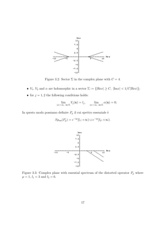
For t = 1, 2, we set ˜pt(x, ξ) = |ξ|2
+ ˜W(x) and
Σt
def
= {(x, ξ) ∈ Rn
× Rn
; ˜pt(x, ξ) ∈ [m2 − 2α, m2 + 2α]}.
We choose χt ∈ C∞
0 ({|x| ≤ 2XC} × Rn
), supported near Σt, such tha χt = 1 in a
neighborhood of Σt. We ﬁx also χ0 = χ0(x) ∈ C∞
0 (|x| ≤ 2XC) such that χ0 = 1 on
{|x| ≤ 2XC}.
Now, using some pseudodiﬀerential calculus, for every E ∈ [m2 − 2α, m2 + 2α] we
can make a symbol qt(E) = qt(E, x, ξ; h), supported in {|x| ≤ 2XC} × Rn
and smooth
with respect to E, such that
qt(E)#(˜pt − E)(x, ξ) ∼ χ0(x)(1 − χt(x, ξ)), (5.8)
where # is Weyl composition of symbols
a#b(x, ξ; h) = eih[DηDx−DθDξ]
a(θ, η)b(x, ξ)|θ=x,η=ξ = a(x, ξ)b(x, ξ)+
h
2i
{a, b}(x, ξ)+O(h2
),
and the asymptotic equivalence holds uniformly with respect to E ∈ [m2 − 2α, m2 + 2α].
We see that ˜pt − E = 0 on the support of χ0(1 − χ1). Then, multiplying (5.6) by χ0,
commuting χ0 with ˜Pj and applying Weyl quantization of qt(E) (with E = E1,j, E2,k
respectively) we deduce from (5.6), (5.7) and (5.8) that
Op(χ0(x)(1 − χ1(x, ξ)))φj Hs = O(h∞
), (5.9)
Op(χ0(x)(1 − χ2(x, ξ)))ψk Hs = O(h∞
) (5.10)
uniformly with respect to j, k. Indeed, for E = E1,j we have 0 = χ0( ˜P1 − E)φj =
[ ˜P1, χ0]φj + ( ˜P1 − E)χ0φj, and as the term [ ˜P1, χ1]φj is exponentially small, then ( ˜P1 −
E)χ0φj is too. Setting Q1 = Op(q1(E)), we have Q1( ˜P1 − E)χ0φj = Op(q1(E)#(˜p1 −
Figure 5.1: Possible Σ1 and Σ2 on phase space.
29

E))χ0φj = Op(χ0(x)(1 − χ1(x, ξ)))χ0φj is exponentially small, and as (1 − χ0)φj is
too, it follows the result for φj. The same reasoning can be repeated for Op(χ0(x)(1 −
χ2(x, ξ)))ψk. Finally, from (5.7) it follows that
(1 − χ1(x, ξ))φj Hs = O(h∞
), (5.11)
(1 − χ2(x, ξ))ψk Hs = O(h∞
). (5.12)
To complete the proof, we introduce the notion of set of frequencies for a function.
Given φ ∈ L2
, we say a point (x0, ξ0) ∈ R2n
doesn’t belong to the set of the frequencies
of φ, and we write (x0, ξ0) /∈ FS(φ), if there exists a function χ ∈ C∞
0 (R2n
) such that
χ = 1 near (x0, ξ0) and χ(x, hDx)φ = O(h∞
). We know that (cfr. [8], proposition
2.9.4) in such a definition the condition ‘there exists a function χ ∈ C∞
0 (R2n
) such that
χ = 1 near (x0, ξ0)’ implies the condition ’for every function χ ∈ C∞
0 (R2n
) supported in a
small enough neighborhood of (x0, ξ0). We also say the function φ is microlocally O(h∞
)
near the point (x0, ξ0). Moreover, if (x0, ξ0) /∈ FS(φ) then for every pseudodifferential
operator A (x0, ξ0) /∈ FS(Aφ), that is, pseudodifferential operators don’t make bigger
the set of the frequencies of a function.
From the previous result, it follows immediately that
FS(Aφj) ⊂ FS(φj) ⊂ Σ1, FS(Aψk) ⊂ FS(ψk) ⊂ Σ2.
Yet, as we can remark from figure (5.1), Σ1 ∩Σ2 = ∅, so FS(Aφj)∩FS(Aψk) = ∅. Then,
φj and Aφj ‘microlocally live’ on Σ1, and both ψk and Aψk on Σ2, and we have
φj = χ1(x, hDx)φj + O(h∞
), ψk = χ2(x, hDx)ψk + O(h∞
),
A0φj = A0χ1(x, hDx)φj + O(h∞
), A0ψk = A0χ2(x, hDx)ψk + O(h∞
),
for every χt ∈ C∞
0 (R2n
) such that χt = 1 near Σt. Now, it remains
A0χ1(x, hDx)φj + O(h∞
) = χ1(x, hDx)A0φj + [A0, χ1(x, hDx)]φj + O(h∞
),
A0χ2(x, hDx)ψk + O(h∞
) = χ2(x, hDx)A0ψk + [A0, χ2(x, hDx)]ψk + O(h∞
),
where the symbols of the commutators can be expanded in a series with coefficients
supported in the support in the that of the gradient of χ1 and χ2 respectively. Yet
Supp χt ∩ Σt = ∅, so
A0φj = χ1(x, hDx)A0φj + O(h∞
), A0ψk = χ2(x, hDx)A0ψk + O(h∞
),
from which, writing χt for χt(x, hDx), it finally follows that
A0φj, ψk = χ1A0φj, χ2ψk + O(h∞
) = χ2χ1A0φj, ψk + O(h∞
) = O(h∞
),
A0ψk, φj = χ2A0ψk, χ1φj + O(h∞
) = χ1χ2A0ψk, φj + O(h∞
) = O(h∞
).
30

In order to complete the proof of the propositiom it suﬃced to show that the matrix
R+
˜PR− − diag(E1,1, . . . , E1,l, E2,1, . . . , E2,m) =
0 ( A0ψk, φj )
( A∗
0φj, ψk ) 0
has dimension O(h−n
) and that the lemma just proved implies it has norm O(h∞
) on
Cl+m
uniformly with respect to n, m. The statement follows from (5.5).
From Min-Max principle and from previous proposition it follows that, for λ ∈ [m2 −
α, m2 + α], the eigenvalues g1(λ), . . . , gl+m(λ) of Q(λ) are such that
i. {g1(λ, . . . , gl+m(λ)} ⊂ {E1,1, . . . , E1,l, E2,1, . . . , E2,m} + O(h2
);
ii. to every E ∈ {E1,1, . . . , E1,l, E2,1, . . . , E2,m} ∩ [m2 − α + Ch2
, m2 + α − Ch2
], with
C >> 1, it can be associated a unique λ ∈ [m2 −α, m2 +α] such that λ ∈ Sp(Q(λ)).
Finally, using the fact that the eigenvalues of ˜P lying in [m2 − α, m2 + α] coincides
by construction with the local solution of λ ∈ Sp(Q(λ)), and remembering the results of
the previous chapters, we get the following
Teorema 5.4. For 0 < h << 1 the resonances of P with real part in [m2 − α, m2 + α]
and imaginary part << |h ln h| coincide, but for a h2
order error term, with eigenvalues
of Dirichlet realizations of P1 and P2 on a open set B ⊂ Rn
which contains the well and
is contained in the isle.
31

Bibliography
[1] D. Benedetto, E. Caglioti, R. Libero, Non-trapping set and Huygens principle,
ESAIM : Modélisation Mathématique et Analyse Numérique, 33 no. 3 (1999), p.
517-530.
[2] M. Born, R. Oppenheimer, Zur Quantentheorie der Molekeln, Ann. Phys. 84
(1927), 457-484.
[3] G. Dell’Antonio, Mathematical Aspects of Quantum Mechanics.
[4] V. Grecchi, H. Kovaˆr`ık, A. Martinez, A. Sacchetti, V. Sordoni, The Stark Effect
on the H+
2 -like Molecules, preprint.
[5] B. Helffer, J. Sjöstrand, Multiple wells in the semiclassical limit I, Comm. Part.
Diff. Eq. 9 (4) (1984) 337-408.
[6] B. Helffer, J. Sjöstrand, Resonances en limite semi-classique, Ann. Inst. Henri
Poincaré, section Physique Théorique, vol. 41, n. 3 (1984), 291-331.
[7] B. Helffer, J. Sjöstrand, Puits multiples en limite-semiclassique. II. Interaction
moléculaaire. Symetries. Perturbation Ann. Inst. Henri Poincaré, section A, vol.
42, n. 2 (1985), 127-212.
[8] A. Martinez, An introduction to Semiclassical and Microlocal Analysis, Springer,
2002, New York.
[9] A. Martinez, Développement asymptotiques ed effet tunnel dans l’approximation
de Born-Oppenheimer, Ann. Inst. H. Poincaré 49 (1989), 239-257.
[10] A. Martinez, Resonance Free Domains for Non Globally Analytic Potentials, Ann.
Henri Poincaré 4 (2002) 739 - 756.
[11] A. Martinez, V. Sordoni, Twisted Pseudodifferential Calculus and Application to
the Quantum Evolution of Molecules, AMS, 2009, Providence (Rhode Island).
33

[12] M. Reed, B. Simon, Methods of Modern Mathematical Physics, II volume, Elsevier,
1975, Amsterdam.
[13] M. Reed, B. Simon, Methods of Modern Mathematical Physics, IV volume, Else-
vier, 1978, Amsterdam.
[14] H. C. Urey, The Structure of the Hydrogen Molecule Ion, 1925, Proc. Natl. Acad.
Sci. U.S.A. 11 (10): 618-21.
[15] Wikipedia, the free encyclopedia.
34

Tesi

More Related Content

What's hot

Viewers also liked

Similar to Tesi

Tesi