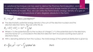
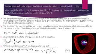
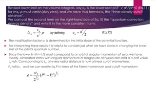
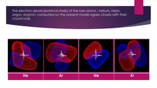
Is Gravitation A Result Of Asymmetric Coulomb Charge Interactions?Jeffrey Gold
Journal of Undergraduate Research (JUR), University of Utah (1992), Vol. 3, No. 1, pp. 56-61.
Jeffrey F. Gold
Department of Physics, Department of Mathematics
University of Utah
Abstract
Many attempts have been made to equate gravitational forces with manifestations of other phenomena. In these remarks we explore the consequences of formulating gravitational forces as asymmetric Coulomb charge interactions. This is contrary to some established theories, for the model predicts differential accelerations dependent on the elemental composition of the test mass. The
predicted di erentials of acceleration of various elemental masses are compared to those differentials that have been obtained experimentally. Although the model turns out to fail, the construction of this model is a useful intellectual and pedagogical exercise.
I am Ben R. I am a Statistics Assignment Expert at statisticshomeworkhelper.com. I hold a Ph.D. in Statistics, from University of Denver, USA. I have been helping students with their homework for the past 5 years. I solve assignments related to Statistics.
Visit statisticshomeworkhelper.com or email info@statisticshomeworkhelper.com.
You can also call on +1 678 648 4277 for any assistance with Statistics Assignment.
I am Joshua M. I am a Statistical Physics Assignment Expert at statisticsassignmenthelp.com. I hold a Masters in Statistics from, Michigan State University, UK
I have been helping students with their homework for the past 5 years. I solve assignments related to Statistics.
Visit statisticsassignmenthelp.com or email info@statisticsassignmenthelp.com.
You can also call on +1 678 648 4277 for any assistance with Statistical Physics Assignments .
In the last set of notes, we developed a model of the speed governing mechanism, which is given below:
(1)
In these notes, we want to extend this model so that it relates the actual mechanical power into the machine (instead of ΔxE), so that we can then examine the relation between the mechanical power into the machine and frequency deviation.
Field energy correction with discrete chargesSergio Prats
This document introduces a correction in the classical electromagnetic field energy density when there are discrete charges instead of a whole density of charge based in the fact that the EM field induces by a particle does not affect itself and does not contribute to the potential in the hamiltonian.
A deeper analysis is done on how to deal with the radiated field energy, the reaction force and its analogy with quan Vacuum
I am Grey N. I am a Chemistry Assignment Expert at eduassignmenthelp.com. I hold a Ph.D. in Chemistry, from Calgary, Canada. I have been helping students with their homework for the past 6 years. I solve assignments related to Chemistry.
Visit eduassignmenthelp.com or email info@eduassignmenthelp.com.
You can also call on +1 678 648 4277 for any assistance with Chemistry Assignments.
Artigo que descreve o trabalho feito com o Chandra nos aglomerados de galáxias de Perseus e Virgo sobre a descoberta de uma turbulência cósmica que impede a formação de novas estrelas.
I am Ben R. I am a Statistics Assignment Expert at statisticshomeworkhelper.com. I hold a Ph.D. in Statistics, from University of Denver, USA. I have been helping students with their homework for the past 5 years. I solve assignments related to Statistics.
Visit statisticshomeworkhelper.com or email info@statisticshomeworkhelper.com.
You can also call on +1 678 648 4277 for any assistance with Statistics Assignments.
By using the anharmonic correlated einstein model to define the expressions o...Premier Publishers
By using potential effective interaction in the anharmonic correlated Einstein model on the basis of quantum statistical theory with phonon interaction procedure, the expressions describing asymmetric component (cumulants) and thermodynamic parameters including the anharmonic effects contributions and by new structural parameters of cubic crystals have been formulated. These new parameters describe the distribution of atoms. The expansion of cumulants and thermodynamic parameters through new structural parameters has been performed. The results of this study show that, developing further the anharmonic correlated Einstein model it obtained a general theory for calculation cumulants and thermodynamic parameters in XAFS theory including anharmonic contributions. The expressions are described through new structural parameters that agree with structural contributions of cubic crystals like face center cubic (fcc), body center cubic (bcc).
1 ECE 6340 Fall 2013 Homework 8 Assignment.docxjoyjonna282
1
ECE 6340
Fall 2013
Homework 8
Assignment: Please do Probs. 1-9 and 13 from the set below.
1) In dynamics, we have the equation
E j Aω= − −∇Φ .
(a) Show that in statics, the scalar potential function Φ can be interpreted as a voltage
function. That is, show that in statics
( ) ( )
B
AB
A
V E dr A B≡ ⋅ = Φ −Φ∫ .
(b) Next, explain why this equation is not true (in general) in dynamics.
(c) Explain why the voltage drop (defined as the line integral of the electric field, as
defined above) depends on the path from A to B in dynamics, using Faraday’s law.
(d) Does the right-hand side of the above equation (the difference in the potential
function) depend on the path, in dynamics?
Hint: Note that, according to calculus, for any function ψ we have
dr dx dy dz d
x y z
ψ ψ ψ
ψ ψ
∂ ∂ ∂
∇ ⋅ = + + =
∂ ∂ ∂
.
2) Starting with Maxwell’s equations, show that the electric field radiated by an impressed
current density source J i in an infinite homogeneous region satisfies the equation
( )2 2 iE k E E j Jωµ∇ + = ∇ ∇⋅ + .
Then use Ampere’s law (or, if you prefer, the continuity equation and the electric Gauss
law) to show that this equation may be written as
( )2 2 1 i iE k E J j J
j
ωµ
σ ωε
∇ + = − ∇ ∇⋅ +
+
.
2
Note that the total current density is the sum of the impressed current density and the
conduction current density, the latter obeying Ohm’s law (J c = σE).
Explain why this equation for the electric field would be harder to solve than the equation
that was derived in class for the magnetic vector potential.
3) Show that magnetic field radiated by an impressed current density source satisfies the
equation
2 2 iH k H J∇ + = −∇× .
Explain why this equation for the magnetic field would be harder to solve than the
equation that was derived in class for the magnetic vector potential.
4) Show that in a homogenous region of space the scalar electric potential satisfies the
equation
2 2
i
v
c
k
ρ
ε
∇ Φ + Φ = − ,
where ivρ is the impressed (source) charge density, which is the charge density that goes
along with the impressed current density, being related by
i ivJ jωρ∇⋅ = −
Hint: Start with E j Aω= − −∇Φ and take the divergence of both sides. Also, take the
divergence of both sides of Ampere’s law and use the continuity equation for the
impressed current (given above) to show that
1 ii v
c c
E J
j
ρ
ωε ε
∇⋅ = − ∇⋅ = .
Note: It is also true from the electric Gauss law that
vE
ρ
ε
∇⋅ = ,
but we prefer to have only an impressed (source) charge density on the right-hand side of
the equation for the potential Φ. In the time-harmonic steady state, assuming a
homogeneous and isotropic region, it follows that ρv = ρvi. That is, there is no charge
3
density arising from the conduction current. (If there were no impressed current sources,
the total charge density would therefore be ze ...
I am Ben R. I am a Statistics Assignment Expert at statisticshomeworkhelper.com. I hold a Ph.D. in Statistics, from University of Denver, USA. I have been helping students with their homework for the past 5 years. I solve assignments related to Statistics.
Visit statisticshomeworkhelper.com or email info@statisticshomeworkhelper.com.
You can also call on +1 678 648 4277 for any assistance with Statistics Assignment.
I am Joshua M. I am a Statistical Physics Assignment Expert at statisticsassignmenthelp.com. I hold a Masters in Statistics from, Michigan State University, UK
I have been helping students with their homework for the past 5 years. I solve assignments related to Statistics.
Visit statisticsassignmenthelp.com or email info@statisticsassignmenthelp.com.
You can also call on +1 678 648 4277 for any assistance with Statistical Physics Assignments .
In the last set of notes, we developed a model of the speed governing mechanism, which is given below:
(1)
In these notes, we want to extend this model so that it relates the actual mechanical power into the machine (instead of ΔxE), so that we can then examine the relation between the mechanical power into the machine and frequency deviation.
Field energy correction with discrete chargesSergio Prats
This document introduces a correction in the classical electromagnetic field energy density when there are discrete charges instead of a whole density of charge based in the fact that the EM field induces by a particle does not affect itself and does not contribute to the potential in the hamiltonian.
A deeper analysis is done on how to deal with the radiated field energy, the reaction force and its analogy with quan Vacuum
I am Grey N. I am a Chemistry Assignment Expert at eduassignmenthelp.com. I hold a Ph.D. in Chemistry, from Calgary, Canada. I have been helping students with their homework for the past 6 years. I solve assignments related to Chemistry.
Visit eduassignmenthelp.com or email info@eduassignmenthelp.com.
You can also call on +1 678 648 4277 for any assistance with Chemistry Assignments.
Artigo que descreve o trabalho feito com o Chandra nos aglomerados de galáxias de Perseus e Virgo sobre a descoberta de uma turbulência cósmica que impede a formação de novas estrelas.
I am Ben R. I am a Statistics Assignment Expert at statisticshomeworkhelper.com. I hold a Ph.D. in Statistics, from University of Denver, USA. I have been helping students with their homework for the past 5 years. I solve assignments related to Statistics.
Visit statisticshomeworkhelper.com or email info@statisticshomeworkhelper.com.
You can also call on +1 678 648 4277 for any assistance with Statistics Assignments.
By using the anharmonic correlated einstein model to define the expressions o...Premier Publishers
By using potential effective interaction in the anharmonic correlated Einstein model on the basis of quantum statistical theory with phonon interaction procedure, the expressions describing asymmetric component (cumulants) and thermodynamic parameters including the anharmonic effects contributions and by new structural parameters of cubic crystals have been formulated. These new parameters describe the distribution of atoms. The expansion of cumulants and thermodynamic parameters through new structural parameters has been performed. The results of this study show that, developing further the anharmonic correlated Einstein model it obtained a general theory for calculation cumulants and thermodynamic parameters in XAFS theory including anharmonic contributions. The expressions are described through new structural parameters that agree with structural contributions of cubic crystals like face center cubic (fcc), body center cubic (bcc).
1 ECE 6340 Fall 2013 Homework 8 Assignment.docxjoyjonna282
1
ECE 6340
Fall 2013
Homework 8
Assignment: Please do Probs. 1-9 and 13 from the set below.
1) In dynamics, we have the equation
E j Aω= − −∇Φ .
(a) Show that in statics, the scalar potential function Φ can be interpreted as a voltage
function. That is, show that in statics
( ) ( )
B
AB
A
V E dr A B≡ ⋅ = Φ −Φ∫ .
(b) Next, explain why this equation is not true (in general) in dynamics.
(c) Explain why the voltage drop (defined as the line integral of the electric field, as
defined above) depends on the path from A to B in dynamics, using Faraday’s law.
(d) Does the right-hand side of the above equation (the difference in the potential
function) depend on the path, in dynamics?
Hint: Note that, according to calculus, for any function ψ we have
dr dx dy dz d
x y z
ψ ψ ψ
ψ ψ
∂ ∂ ∂
∇ ⋅ = + + =
∂ ∂ ∂
.
2) Starting with Maxwell’s equations, show that the electric field radiated by an impressed
current density source J i in an infinite homogeneous region satisfies the equation
( )2 2 iE k E E j Jωµ∇ + = ∇ ∇⋅ + .
Then use Ampere’s law (or, if you prefer, the continuity equation and the electric Gauss
law) to show that this equation may be written as
( )2 2 1 i iE k E J j J
j
ωµ
σ ωε
∇ + = − ∇ ∇⋅ +
+
.
2
Note that the total current density is the sum of the impressed current density and the
conduction current density, the latter obeying Ohm’s law (J c = σE).
Explain why this equation for the electric field would be harder to solve than the equation
that was derived in class for the magnetic vector potential.
3) Show that magnetic field radiated by an impressed current density source satisfies the
equation
2 2 iH k H J∇ + = −∇× .
Explain why this equation for the magnetic field would be harder to solve than the
equation that was derived in class for the magnetic vector potential.
4) Show that in a homogenous region of space the scalar electric potential satisfies the
equation
2 2
i
v
c
k
ρ
ε
∇ Φ + Φ = − ,
where ivρ is the impressed (source) charge density, which is the charge density that goes
along with the impressed current density, being related by
i ivJ jωρ∇⋅ = −
Hint: Start with E j Aω= − −∇Φ and take the divergence of both sides. Also, take the
divergence of both sides of Ampere’s law and use the continuity equation for the
impressed current (given above) to show that
1 ii v
c c
E J
j
ρ
ωε ε
∇⋅ = − ∇⋅ = .
Note: It is also true from the electric Gauss law that
vE
ρ
ε
∇⋅ = ,
but we prefer to have only an impressed (source) charge density on the right-hand side of
the equation for the potential Φ. In the time-harmonic steady state, assuming a
homogeneous and isotropic region, it follows that ρv = ρvi. That is, there is no charge
3
density arising from the conduction current. (If there were no impressed current sources,
the total charge density would therefore be ze ...
A free electron model is the simplest way to represent the
electronic structure and properties of metals.
According to this model, the valence electrons of the constituent
atoms of the crystal become conduction electrons and travel
freely throughout the crystal.
The classical theory fails to explain the heat capacity and the
magnetic susceptibility of the conduction electrons. (These are
not failures of the free electron model, but failures of the classical
Maxwell distribution function.)
Condensed matter is so transparent to conduction electrons
The fundamental theory of electromagnetic field is based on Maxwell.pdfinfo309708
The fundamental theory of electromagnetic field is based on Maxwell\'s equations. These
equations govern the electromagnetic fields, E, D, H, and there relations to the source, f and p_v.
In a source-free region, list the Maxwell\'s equations for time-harmonic fields: Given the Phaser
from of the electric field E? For the above given electric field, is B varying with time? Why?
Solution
Maxwell’s equations simplify considerably in the case of harmonic time dependence. Through
the inverse Fourier transform, general solutions of Maxwell’s equation can be built as linear
combinations of single-frequency solutions:† E(r, t)= E(r, )ejt d2 (1) Thus, we assume that all
fields have a time dependence ejt: E(r, t)= E(r)ejt, H(r, t)= H(r)ejt where the phasor amplitudes
E(r), H(r) are complex-valued. Replacing time derivatives by t j, we may rewrite Eq. in the
form:
× E = jB
× H = J + jD
· D =
· B = 0
(Maxwell’s equations) (2) In this book, we will consider the solutions of Eqs. (.2) in three
different contexts: (a) uniform plane waves propagating in dielectrics, conductors, and
birefringent media, (b) guided waves propagating in hollow waveguides, transmission lines, and
optical fibers, and (c) propagating waves generated by antennas and apertures
Next, we review some conventions regarding phasors and time averages. A realvalued sinusoid
has the complex phasor representation: A(t)= |A| cos(t + ) A(t)= Aejt (3) where A = |A|ej. Thus,
we have A(t)= Re A(t) = Re Aejt . The time averages of the quantities A(t) and A(t) over one
period T = 2/ are zero. The time average of the product of two harmonic quantities A(t)= Re Aejt
and B(t)= Re Bejt with phasors A, B is given by A(t)B(t) = 1T T0 A(t)B(t) dt = 12 Re AB] (4) In
particular, the mean-square value is given by: A2(t) = 1T T0 A2(t) dt = 12 Re AA]= 12|A|2 (5)
Some interesting time averages in electromagnetic wave problems are the time averages of the
energy density, the Poynting vector (energy flux), and the ohmic power losses per unit volume.
Using the definition) and the result (.4), we have for these time averages:
w = 1 2 Re 12E · E + 12H · H (energy density) P = 1/ 2 Re E × H (Poynting vector) dPloss dV =
1/ 2 Re Jtot · E (ohmic losses) (6) where Jtot = J + jD is the total current in the right-hand side of
Amp`ere’s law and accounts for both conducting and dielectric losses. The time-averaged
version of Poynting’s theorem is discussed in Problem 1.5. The expression (1.9.6) for the energy
density w was derived under the assumption that both and were constants independent of
frequency. In a dispersive medium, , become functions of frequency. In frequency bands where
(), () are essentially real-valued, that is, where the medium is lossless,that the timeaveraged
energy density generalizes to: w = 1/ 2 Re 1/2 d() d E · E + 1/2 d() d H · H (lossless case) (.7)
The derivation of (.7) is as follows. Starting with Maxwell’s equations (1.1.1) and without
assuming any particular constitutive relations, we obtain:.
The fundamental theory of electromagnetic field is based on Maxwell.pdfRBMADU
The fundamental theory of electromagnetic field is based on Maxwell\'s equations. These
equations govern the electromagnetic fields, E, D, H, and there relations to the source, f and p_v.
In a source-free region, list the Maxwell\'s equations for time-harmonic fields: Given the Phaser
from of the electric field E? For the above given electric field, is B varying with time? Why?
Solution
Maxwell’s equations simplify considerably in the case of harmonic time dependence. Through
the inverse Fourier transform, general solutions of Maxwell’s equation can be built as linear
combinations of single-frequency solutions:† E(r, t)= E(r, )ejt d2 (1) Thus, we assume that all
fields have a time dependence ejt: E(r, t)= E(r)ejt, H(r, t)= H(r)ejt where the phasor amplitudes
E(r), H(r) are complex-valued. Replacing time derivatives by t j, we may rewrite Eq. in the
form:
× E = jB
× H = J + jD
· D =
· B = 0
(Maxwell’s equations) (2) In this book, we will consider the solutions of Eqs. (.2) in three
different contexts: (a) uniform plane waves propagating in dielectrics, conductors, and
birefringent media, (b) guided waves propagating in hollow waveguides, transmission lines, and
optical fibers, and (c) propagating waves generated by antennas and apertures
Next, we review some conventions regarding phasors and time averages. A realvalued sinusoid
has the complex phasor representation: A(t)= |A| cos(t + ) A(t)= Aejt (3) where A = |A|ej. Thus,
we have A(t)= Re A(t) = Re Aejt . The time averages of the quantities A(t) and A(t) over one
period T = 2/ are zero. The time average of the product of two harmonic quantities A(t)= Re Aejt
and B(t)= Re Bejt with phasors A, B is given by A(t)B(t) = 1T T0 A(t)B(t) dt = 12 Re AB] (4) In
particular, the mean-square value is given by: A2(t) = 1T T0 A2(t) dt = 12 Re AA]= 12|A|2 (5)
Some interesting time averages in electromagnetic wave problems are the time averages of the
energy density, the Poynting vector (energy flux), and the ohmic power losses per unit volume.
Using the definition) and the result (.4), we have for these time averages:
w = 1 2 Re 12E · E + 12H · H (energy density) P = 1/ 2 Re E × H (Poynting vector) dPloss dV =
1/ 2 Re Jtot · E (ohmic losses) (6) where Jtot = J + jD is the total current in the right-hand side of
Amp`ere’s law and accounts for both conducting and dielectric losses. The time-averaged
version of Poynting’s theorem is discussed in Problem 1.5. The expression (1.9.6) for the energy
density w was derived under the assumption that both and were constants independent of
frequency. In a dispersive medium, , become functions of frequency. In frequency bands where
(), () are essentially real-valued, that is, where the medium is lossless,that the timeaveraged
energy density generalizes to: w = 1/ 2 Re 1/2 d() d E · E + 1/2 d() d H · H (lossless case) (.7)
The derivation of (.7) is as follows. Starting with Maxwell’s equations (1.1.1) and without
assuming any particular constitutive relations, we obtain:.
Stellar Measurements with the New Intensity FormulaIOSR Journals
In this paper a linear relationship in stellar optical spectra has been found by using a
spectroscopical method used on optical light sources where it is possible to organize atomic and ionic data.
This method is based on a new intensity formula in optical emission spectroscopy (OES). Like the HR-diagram ,
it seems to be possible to organize the luminosity of stars from different spectral classes. From that organization
it is possible to determine the temperature , density and mass of stars by using the new intensity formula. These
temperature, density and mass values agree well with literature values. It is also possible to determine the mean
electron temperature of the optical layers (photospheres) of the stars as it is for atoms in the for laboratory
plasmas. The mean value of the ionization energies of the different elements of the stars has shown to be very
significant for each star. This paper also shows that the hydrogen Balmer absorption lines in the stars follow
the new intensity formula.
The Propagation and Power Deposition of Electron Cyclotron Waves in Non-Circu...IJERA Editor
By solving the plasma equilibrium equation, ray equations, and quasi-linear Fokker-Planck equation, the ray
trajectories and power deposition of EC wave has been numerically simulated in non-circular HL-2A tokamak
plasma. The results show that shaping effect and temperature profile has little influence on ECRH, while plasma
density affect propagation and power deposition obviously. when the ordinary mode of EC waves are launched
from the mid-plane and low-field-side, ray trajectories are bended as the parallel refractive index increases and
even recurve to the low-field side when the parallel refractive index reaches to a certain value. Single absorption
decreases with increasing both poloidal and toroidal injection angle, and can be 100% when poloidal injection
angle is 180o and toroidal injection angle is less than 10o.
Similar to Sergey seriy thomas fermi-dirac theory (20)
Slack (or Teams) Automation for Bonterra Impact Management (fka Social Soluti...Jeffrey Haguewood
Sidekick Solutions uses Bonterra Impact Management (fka Social Solutions Apricot) and automation solutions to integrate data for business workflows.
We believe integration and automation are essential to user experience and the promise of efficient work through technology. Automation is the critical ingredient to realizing that full vision. We develop integration products and services for Bonterra Case Management software to support the deployment of automations for a variety of use cases.
This video focuses on the notifications, alerts, and approval requests using Slack for Bonterra Impact Management. The solutions covered in this webinar can also be deployed for Microsoft Teams.
Interested in deploying notification automations for Bonterra Impact Management? Contact us at sales@sidekicksolutionsllc.com to discuss next steps.
"Impact of front-end architecture on development cost", Viktor TurskyiFwdays
I have heard many times that architecture is not important for the front-end. Also, many times I have seen how developers implement features on the front-end just following the standard rules for a framework and think that this is enough to successfully launch the project, and then the project fails. How to prevent this and what approach to choose? I have launched dozens of complex projects and during the talk we will analyze which approaches have worked for me and which have not.
PHP Frameworks: I want to break free (IPC Berlin 2024)Ralf Eggert
In this presentation, we examine the challenges and limitations of relying too heavily on PHP frameworks in web development. We discuss the history of PHP and its frameworks to understand how this dependence has evolved. The focus will be on providing concrete tips and strategies to reduce reliance on these frameworks, based on real-world examples and practical considerations. The goal is to equip developers with the skills and knowledge to create more flexible and future-proof web applications. We'll explore the importance of maintaining autonomy in a rapidly changing tech landscape and how to make informed decisions in PHP development.
This talk is aimed at encouraging a more independent approach to using PHP frameworks, moving towards a more flexible and future-proof approach to PHP development.
Neuro-symbolic is not enough, we need neuro-*semantic*Frank van Harmelen
Neuro-symbolic (NeSy) AI is on the rise. However, simply machine learning on just any symbolic structure is not sufficient to really harvest the gains of NeSy. These will only be gained when the symbolic structures have an actual semantics. I give an operational definition of semantics as “predictable inference”.
All of this illustrated with link prediction over knowledge graphs, but the argument is general.
UiPath Test Automation using UiPath Test Suite series, part 3DianaGray10
Welcome to UiPath Test Automation using UiPath Test Suite series part 3. In this session, we will cover desktop automation along with UI automation.
Topics covered:
UI automation Introduction,
UI automation Sample
Desktop automation flow
Pradeep Chinnala, Senior Consultant Automation Developer @WonderBotz and UiPath MVP
Deepak Rai, Automation Practice Lead, Boundaryless Group and UiPath MVP
Connector Corner: Automate dynamic content and events by pushing a buttonDianaGray10
Here is something new! In our next Connector Corner webinar, we will demonstrate how you can use a single workflow to:
Create a campaign using Mailchimp with merge tags/fields
Send an interactive Slack channel message (using buttons)
Have the message received by managers and peers along with a test email for review
But there’s more:
In a second workflow supporting the same use case, you’ll see:
Your campaign sent to target colleagues for approval
If the “Approve” button is clicked, a Jira/Zendesk ticket is created for the marketing design team
But—if the “Reject” button is pushed, colleagues will be alerted via Slack message
Join us to learn more about this new, human-in-the-loop capability, brought to you by Integration Service connectors.
And...
Speakers:
Akshay Agnihotri, Product Manager
Charlie Greenberg, Host
Builder.ai Founder Sachin Dev Duggal's Strategic Approach to Create an Innova...Ramesh Iyer
In today's fast-changing business world, Companies that adapt and embrace new ideas often need help to keep up with the competition. However, fostering a culture of innovation takes much work. It takes vision, leadership and willingness to take risks in the right proportion. Sachin Dev Duggal, co-founder of Builder.ai, has perfected the art of this balance, creating a company culture where creativity and growth are nurtured at each stage.
The Art of the Pitch: WordPress Relationships and SalesLaura Byrne
Clients don’t know what they don’t know. What web solutions are right for them? How does WordPress come into the picture? How do you make sure you understand scope and timeline? What do you do if sometime changes?
All these questions and more will be explored as we talk about matching clients’ needs with what your agency offers without pulling teeth or pulling your hair out. Practical tips, and strategies for successful relationship building that leads to closing the deal.
Smart TV Buyer Insights Survey 2024 by 91mobiles.pdf91mobiles
91mobiles recently conducted a Smart TV Buyer Insights Survey in which we asked over 3,000 respondents about the TV they own, aspects they look at on a new TV, and their TV buying preferences.
Knowledge engineering: from people to machines and back
Sergey seriy thomas fermi-dirac theory
1. Modern ab-initio calculations
based on Tomas-Fermi-Dirac
theory with quantum,
correlation and multishells
corrections
SERGEY SERIY, PH.D., EMAIL: SERGGRAY@MAIL.RU
KOMSOMOLSK-ON-AMUR STATE TECHNICAL UNIVERSITY, RUSSIAN FEDERATION
2. A variational technique can be used to derive the Thomas-Fermi equation, and an
extension of this method provides an often-used and simple means of adding corrections
to the statistical model. Thus, we can write the Fermi kinetic energy density of a gas of
free electrons at a temperature of zero degrees absolute in the form:
The electrostatic potential energy density is the sum of the electron-nuclear and the
electron-electron terms. We can write this as
3
5
ff cU where cf=(3/10)(3π2)2/3
)
2
(
e
ne
p
n
pp
v
vUUE
Where vn is the potential due to the nucleus of charge Z, ve is the potential due to the electrons,
and the factor of 1/2 is included in the electron-electron term to avoid counting each pair of
electrons twice.
With x denoting distance from the nucleus, the total energy of the spherical distribution is given by
dxx
v
vcE
e
n
f
23
5
4))
2
(( (Eq.1)
3. The expression for density on the Thomas-Fermi model, ρ=σ0(E’-V)3/2 (Eq.2)
with σ0=(3/5 cf)3/2, is obtained by minimizing Eq.1 subject to the auxiliary condition that
the total number of particles N, remains constant.
The potential energy V, is a function of position in the electron distribution. E’ is the Fermi energy, or
chemical potential, and is constant throughout a given distribution. The Thomas-Fermi equation follows
from Eq.2 and Poisson’s equation.
The tendency for electrons of like spin to stay apart because of exclusion principle is accounted for by
the inclusion in Eq.1 of exchange energy, the volume density of which is given by:
3
4
exex cU , where cex=(3/4)(3/π)1/3
Minimization of the total energy now leads to the equation
0)'(
3
4
3
5 3
1
3
2
VEcc exf
Which is quadratic in ρ1/3. From this equation we get
))'(( 32
000 jVE , where
f
ex
c
c
15
4 2
0 (Eq.3)
4. Now Poisson equation with the density given by Eq.3 leads to the
Thomas-Fermi-Dirac equation.
In the following two slides we propose additional energy terms to be included in Eq.l.
The incorporation of these terms leads to a simple quantum- and correlation-corrected
TFD equation.
The quantum-correction energy density follows from a slight change in the derivation due to March
and Plaskett.
March and Plaskett have demonstrated that the TF approximation to the sum of one-electron
eigenvalues in a spherically symmetric potential is given by the integral:
dldnlnElI rr ),()12(2 (Eq.4)
where the number of states over which the sum is carried is written as
dldnlN r)12(2 (Eq.5)
Here E(nr,l) is the expression for the WKB(quasi-classic) eigenvalues considered as functions of
continuous variables;
nr is the radial quantum number;
l is the orbital quantum number;
and the region of integration is bounded by n = -1/2, l= -1/2, and E(n ,l)=E’.
5. We have included a factor of two in these equations to account for the spin
degeneracy of the electronic states. The Fermi energy E’ is chosen so that Eq.5 gives the
total number of states being considered, the N electrons occupying the N lowest states.
With considerable manipulation, Eq.4 becomes TF energy equation:
and Eq.5 reveals the TF density through the expression
dxx
P
V
P
I 2
2
32
4
3
)
25
3
(
(Eq.6)
dxx
P
N 2
2
3
4
3
(Eq.7)
both integrals being taken between the roots of E’=V(x). We have written these results in atomic
units, so that P, the Fermi momentum, is defined by
)'(2 VEP
It is pertinent to examine the error in the TF sum of eigenvalues, as given by Eq.6, for the case of the
pure Coulomb field. The WKB eigenvalues in a Coulomb field are given by
2
, )
)1(2
(
ln
z
E
r
lnr
6. And let us consider the levels filled from n=1 to n=v, where n is the total quantum
number defined by n=nr+l+1.
Then, for any value of v we can evaluate the error in the TF approximation to the sum of
eigenvalues, comparing always with the correct value, -Z2v. Scott correction to the total
binding energy is obtained by letting v become very large.
Although the sum of one-electron eigenvalues is not the total energy of the statistical atom
because of the electron-electron interaction being counted twice, we might expect to improve
the calculated binding energy greatly by correcting this sum in some manner, since the chief
cause of the discrepancy is certainly the large error in the electron-nuclear potential energy.
This correction can be performed by imposing a new lower limit on l in the integrations above.
When we introduce a new lower limit lmin and a related quantity which we call the “modification
factor”,
2
1
min la
we obtain, after more manipulation, slightly different expressions corresponding to Eq.6 and Eq.7.
From these revised expressions we can identify a quantum-corrected TF density expression,
2
3
2
2
0 )
2
'(
x
a
VE (Eq.9) ,and a corrected kinetic energy density, 2
2
3
5
2x
a
cU fk (Eq.10)
7. Revised lower limit on the volume integrals, say x1, is the lower root of E’-V-a2/2x2=0 (Eq.11)
for x<xl, ρ must vanish(stay zero), and we have thus termed x1 the “inner density cutoff
distance”.
We can call the second term on the right-hand side of Eq.10 the “quantum-correction
energy density” and write it in the more consistent form:
The modification factor a, is determined by the initial slope of the potential function.
For interpreting these results it is helpful to consider just what we have done in changing the lower
limit of the orbital quantum number.
Since the lower limit l=-1/2 must correspond to an orbital angular momentum of zero, we have,
clearly, eliminated states with angular momentum of magnitude between zero and a cutoff value
Lc=aħ. Corresponding to Lc at every radial distance is now a linear cutoff momentum:
Pc=aħ/x , and we can rewrite Eq.9 in terms of the Fermi momentum and cutoff momentum:
2
x
c
U
q
q ,by defining
2
2
acq (Eq.12)
2
3
22
2
3
0
)(
2
cPP
8. At radial distances less than xl, momenta are prohibited over the entire range from zero to
P, so the electron density vanishes.
This interpretation must be modified somewhat when exchange and correlation effects
are included; for then the Fermi momentum is no longer simply given by Eq.8, except very
near the nucleus.
We can define x1 as in the absence of interactions, i.e., as the lower of the roots of Eq.11, but it is not
correct to demand that the density vanish at the upper root. Instead, we require only that the
density be real.
Correlation Correction. The original TF equation describes a system of independent particles, while
the introduction of exchange energy, which leads to the TED equation, represents a correction for
the correlated motion of electrons of like spin. The remainder of the energy of the electron gas is
termed the correlation energy, by its inclusion we are recognizing that electrons, regardless of spin
orientation, tend to avoid one another.
In extensions of the statistical model there have been suggested at least two different expressions,
for the correlation energy that approach, in the appropriate limits, Wigner’s low-density formula and
the expression due to Gell-Mann and Brueckner at high densities. In addition to these, Gombas and
Tomishima have utilized expansions of the correlation energy per particle in powers of ρ1/3 about the
particle density encountered at the outer boundary of the atom or ion. In this expansion, the term of
first-order can be considered as a correction to the exchange energy, and it follows that the TFD
solutions for a given Z then correspond to correlation-corrected solutions for a modified value of Z.
9. Aside from rather poor approximation of the correlation energy, a drawback to this
procedure is that the TFD solutions must be at hand. If solutions representing specified
degrees of compression are desired, the method would appear to be impractical.
It is interesting and fortunate that over density range of interest it is apparently possible to
approximate the correlation energy per particle quite closely by an expression of form:
Where we have set cc = 0.0842, and compared this approximation with the values due to
Carr and Maradudin.
Derivation. From the results of the preceding slides, we can now express the total energy
per unit volume of the charge distribution in the form:
6
1
cc cu
2
3
4
3
5
)
2
(6
7
x
cv
vcccU
q
e
n
cexf
Where all quantities appearing in the equation have been previously defined. By minimizing the
integral of U over the volume occupied by the charge, while requiring that the total number of
electrons be fixed, we obtain the following equation:
0
4
6
1
0
3
1
1
3
2
R
,where
f
ex
c
c
5
4
1 3
2
00
6
7
cc )'(4 2
3
2
0
x
c
VER
q
(Eq.14)
10. The electron density is found as a function of R by solving Eq.14, a quartic in ρ1/6.
To accomplish this we write a “resolvent cubic equation” in terms of another variable, say y:
y3+τ1y2+Ry+(τ1R-υ0
2)=0 . (Eq.15)
Let us use the same symbol y, to denote any real root of this cubic equation.
We can then express the four roots of the quartic, and hence four expressions for the electron
density, in terms of y. One of these expressions possesses the proper behavior in reducing to
previously obtained results in the neglect of correlation and exchange effects, namely:
32
1 )(
8
1
Ry (Eq.16), where )2( 2
11 Ryyy (Eq.17)
We note that ψ vanishes when correlation is neglected, since y=-τ1 is then root of Eq.15. In the familiar
manner we now define a modified TFD potential function θ by the relation: Zθ=(E’-V+τ0
2)x (Eq.18)
and from Poisson equation and Eq.16 we obtain
.;0
,;)(
2
1
1
32
1
xx
xxRy
Z
x
(Eq.19), in terms of θ, )
2
(4 2
02
2
3
2
0
x
a
x
Z
R (Eq.20)
11. Eq.20, Eq.15, Eq.17, and Eq.19 constitute the differential relationship to be satisfied at each
step in the integration. We could, of course, write immediately the solutions of Eq.15 in
analytic form, but it proves convenient in the numerical treatment to obtain a root by the
Newton-Raphson method, since a good first guess in the iteration is available from the
previous integration step.
The boundary conditions on Eq.19 are:
First - as the nucleus is approached the potential must become that the nucleus alone, or
θ(0)=1,
Second – at the outer boundary x2, of the distribution of N electrons,
2
1
2
1
2
4
x
x
x
x
xdxZdxxN
Integration by parts yields
Z
N
x x
x 2
1
)( ,and since ),(1)( 111 xxx
we have the usual condition:
Z
NZ
xxx
)()( 222 (Eq.21)
12. In addition to potential and density distributions, total binding energies of atoms are of
special interest to us here. For the proper evaluation of energies, the arbitrary constant
that is present originally in both the electrostatic potential energy and the Fermi energy
must be specified. The state of infinite separation of the constituent particles is normally
taken to have zero energy.
We therefore follow the usual convention and fix the potential at the edge of the neutral atom at
zero for all values of x2. For an ion the potential energy of an electron at the boundary is taken as:
2x
NZ
V
The defining relation, Eq.18, now gives at the boundary:
or, solving for the Fermi energy,
The total electron-nuclear potential energy is given by
While for the electron-electron potential energy we have
2
2
0
2
2 )()( x
x
NZ
ExZ
2
0
22
2 )(
x
NZ
x
x
ZE
2
1
2
4
x
x
n
p dxx
x
Z
E
2
1
2
4
2
1
x
x
ee
p dxxvE
13. From Eq.18 and the relation V=-(vn+ve), this becomes:
Other energy integrals are, with an obvious notation:
)4(
2
1 2
1
22
0
x
x
n
p
e
p dxx
x
Z
NENEE
dxxcE ff
23
5
4
dxx
x
cE qq
2
2
4
dxxcE exex
23
4
4
dxxcE cc
26
7
4
14. Results. It was pointed out in the introduction that the quantum-corrected
TFD equation yields atomic binding energies in good agreement with
experimental values and with the results of Hartree-Fock calculations:
Z ETFD (a.u.) EHFS (a.u.) Eexp (a.u.)
2 -2.958 -2.878 -2.903
3 -7.601 -7.226 -7.476
4 -14.944 -14.255 -14.665
5 -25.319 -24.079 -24.652
6 -38.995 -37.079 -37.846
7 -56.225 -53.587 -54.589
15. The electron density(external shells) of the rare atoms - helium, neon,
argon, krypton, computed on the present model agree closely with their
crystal radii.
He Ar Ne Kr
16. Thank you for you attention!
Conclusions:
“Keldysh Institute of Applied Mathematic”, Moscow, Russian Federation
“Tohocu University”, Sendai city, Japan