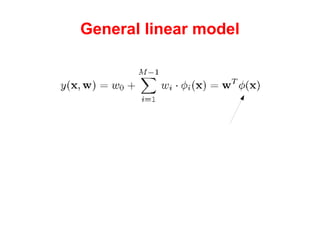
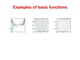
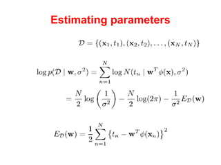
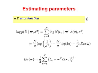
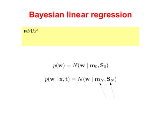
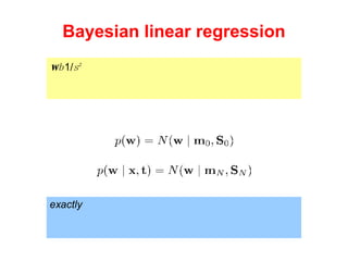
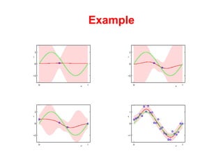
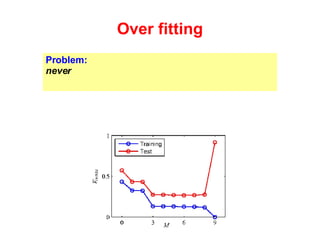
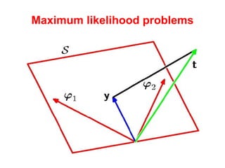
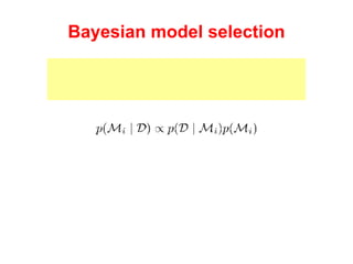
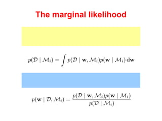
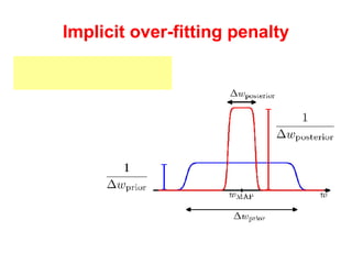
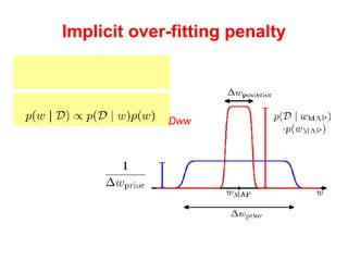
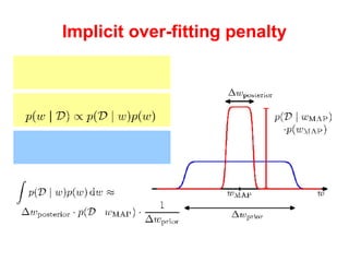
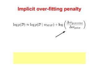
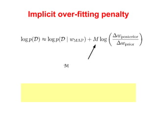
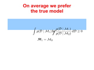
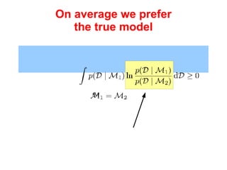
The document discusses linear regression machine learning models. It describes modeling data using a linear Gaussian distribution and estimating the model parameters using maximum likelihood or Bayesian methods. Bayesian estimation avoids the overfitting problems of maximum likelihood estimation by implicitly penalizing models that overfit the data. However, Bayesian methods can still be affected by using an incorrectly specified model.

1. Linear regression Machine Learning; Mon Apr 21, 2008

2. Motivation

3. Motivation Prediction for target? New observed predictor value

4. Motivation Problem: We want a general way of obtaining a distribution p ( x , t ) fitted to observed data. If we don't try to interpret the distribution, then any distribution with non-zero value at the data points will do. We will use theory from last week to construct generic approaches to learning distributions from data.

5. Motivation Problem: We want a general way of obtaining a distribution p ( x , t ) fitted to observed data. If we don't try to interpret the distribution, then any distribution with non-zero value at the data points will do. We will use theory from last week to construct generic approaches to learning distributions from data. In this lecture: linear (normal/Gaussian) models.

6. Linear Gaussian Models In a linear Guassian model, we model p ( x , t ) as a conditional Guassian distribution where the x dependent mean depends linearly on a set of weights w .

7. Example

8. Example

9. General linear in input ...or adding a pseudo input x 0 =1

10. Non-linear in input (but still in weights)

11. Non-linear in input (but still in weights) But remember that we do not know the “true” underlying function...

12. Non-linear in input (but still in weights) ...nor the noise around the function...

13. General linear model Basis functions. Sometimes called “features”.

14. Examples of basis functions Polynomials Gaussians Sigmoids

15. Estimating parameters Log likelihood: Observed data:

16. Estimating parameters Log likelihood: Maximizing wrt w means minimizing E – the error function . Observed data:

17. Estimating parameters

18. Estimating parameters

19. Estimating parameters Notice: This is not just pure mathematics but an actual algorithm for estimating (learning) the parameters!

20. Estimating parameters Notice: This is not just pure mathematics but an actual algorithm for estimating (learning) the parameters! C with GSL and CBLAS

21. Estimating parameters Notice: This is not just pure mathematics but an actual algorithm for estimating (learning) the parameters! Octave/ Matlab

22. Geometrical interpretation Geometrically y is the projection of t onto the space spanned by the features:

23. Bayesian linear regression For the Bayesian approach we need a prior over the parameters w and b = 1/ s 2 Conjugate for Gaussian is Gaussian: Functions of observed values

24. Bayesian linear regression For the Bayesian approach we need a prior over the parameters w and b = 1/ s 2 Conjugate for Gaussian is Gaussian: Proof not exactly like before, but similar, and uses linearity results from Gaussians' from 2.3.3.

25. Example

26. Bayesian linear regression Predictor for future observations is also Guassian (again result from 2.3.3):

27. Bayesian linear regression Predictor for future observations is also Guassian (again result from 2.3.3):

28. Bayesian linear regression Predictor for future observations is also Guassian (again result from 2.3.3): Both mean and variance of this distribution depends on y !

29. Example

30. Over fitting Problem: Over-fitting is always a problem when we fit data to generic models. With nested models, the ML parameters will never prefer a simple model over a more complex model...

31. Maximum likelihood problems

32. Bayesian model selection We can take a more Bayesian approach and select model based on posterior model probabilities:

33. Bayesian model selection We can take a more Bayesian approach and select model based on posterior model probabilities: The normalizing factor is the same for all models:

34. Bayesian model selection We can take a more Bayesian approach and select model based on posterior model probabilities: The prior captures our preferences in the models.

35. Bayesian model selection We can take a more Bayesian approach and select model based on posterior model probabilities: The likelihood captures the data's preferences in models.

36. The marginal likelihood The likelihood of the model is the integral over all the models parameters:

37. The marginal likelihood The likelihood of the model is the integral over all the models parameters: which is also the normalizing factor for the posterior:

38. Implicit over-fitting penalty Assume this is the shape of prior and posterior prior posterior

39. Implicit over-fitting penalty Assume this is the shape of prior and posterior By proportionality prior p( D | w )p( w )

40. Implicit over-fitting penalty Assume this is the shape of prior and posterior By proportionality Integral approximately “width” times “height”

41. Implicit over-fitting penalty Increasingly negative as posterior becomes “pointy” compared to prior Close fitting to data is implicitly penalized, and the marginal likelihood is a trade-off between maximizing the posterior and minimizing this penalty.

42. Implicit over-fitting penalty Penalty increases with number of parameters M Close fitting to data is implicitly penalized, and the marginal likelihood is a trade-off between maximizing the posterior and minimizing this penalty.

43. On average we prefer the true model Penalty increases with number of parameters M This doesn't mean we always prefer the simplest model! One can show with zero only when i.e. on average the right model is the preferred model.

44. On average we prefer the true model Penalty increases with number of parameters M This doesn't mean we always prefer the simplest model! One can show with zero only when i.e. on average the right model is the preferred model. Negative when we prefer the second model positive when we prefer the first

45. On average we prefer the true model Penalty increases with number of parameters M This doesn't mean we always prefer the simplest model! One can show with zero only when i.e. on average the right model is the preferred model. On average, we will not prefer the second model when the first is true...

46. On average we prefer the true model Penalty increases with number of parameters M Close fitting to data is implicitly penalized, and the marginal likelihood is a trade-off between maximizing the posterior and minimizing this penalty. This doesn't mean we always prefer the simplest model! One can show with zero only when i.e. on average the right model is the preferred model.

47. On average we prefer the true model

48. Summary Linear Gaussians as generic densities ML or Bayesian estimation for training Over-fitting is an inherent problem in ML estimation Bayesian methods avoid the maximization caused over-fitting problem (but is still vulnerable to model mis-specification)