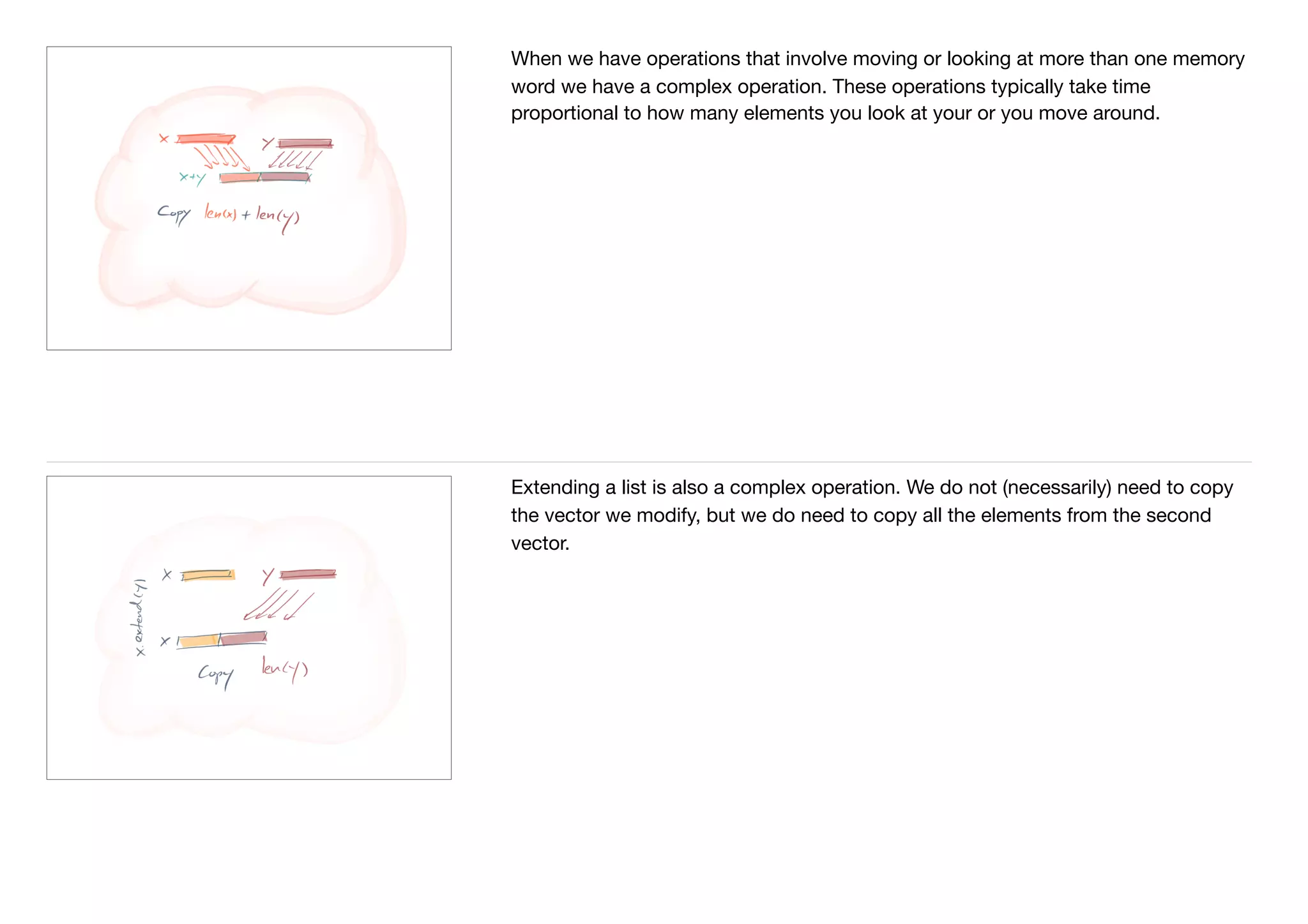
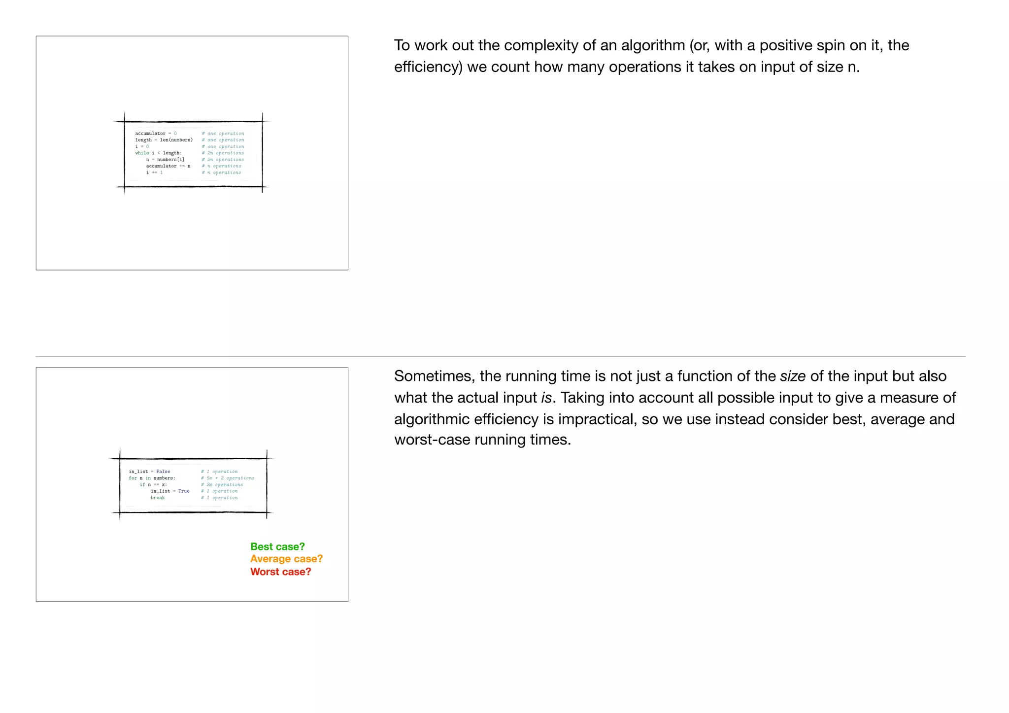
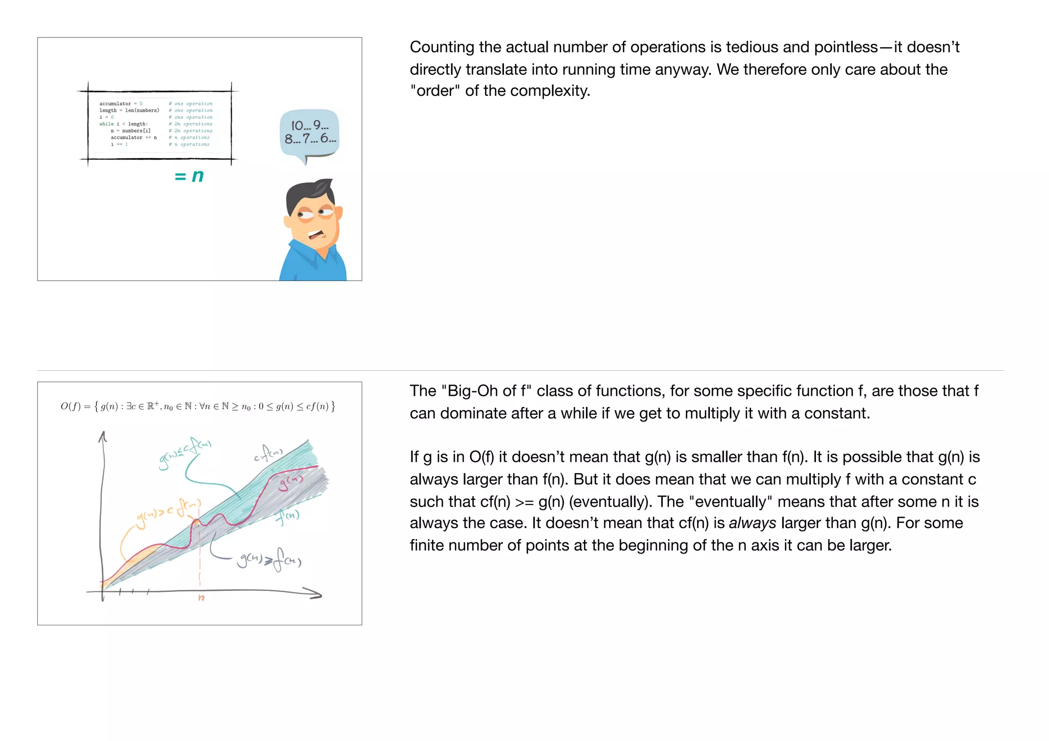
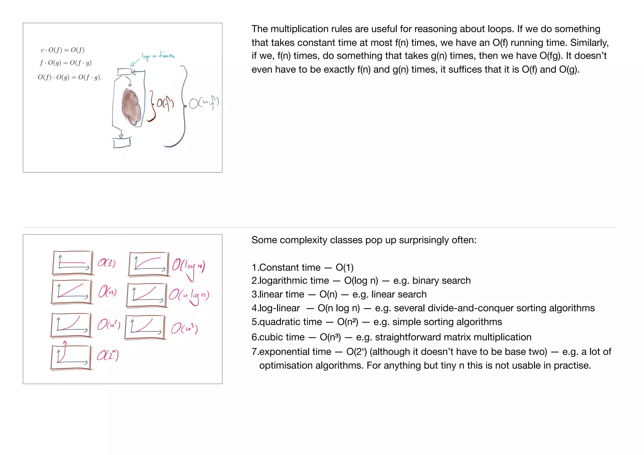
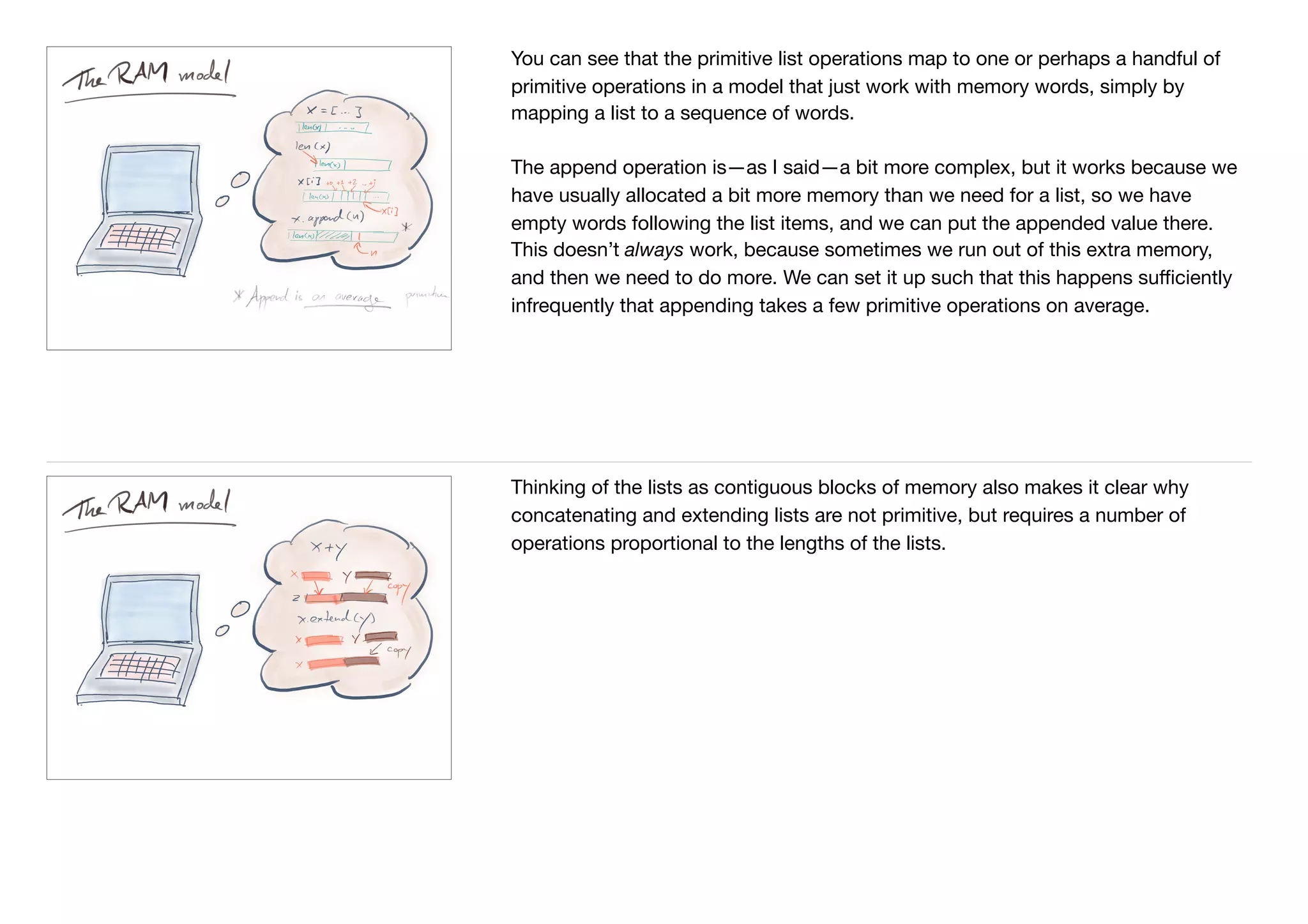
The document discusses algorithmic complexity and the RAM model for analyzing computational efficiency. It explains that the RAM model treats memory as contiguous words that can be accessed and stored values in primitive operations. Common data structures like lists can be modeled in this way. The complexity of operations like concatenating lists, deleting elements, or extending lists is analyzed based on the number of primitive operations required. The document also covers analyzing best, average, and worst-case complexity and discusses common complexity classes like constant, logarithmic, linear, and quadratic time.
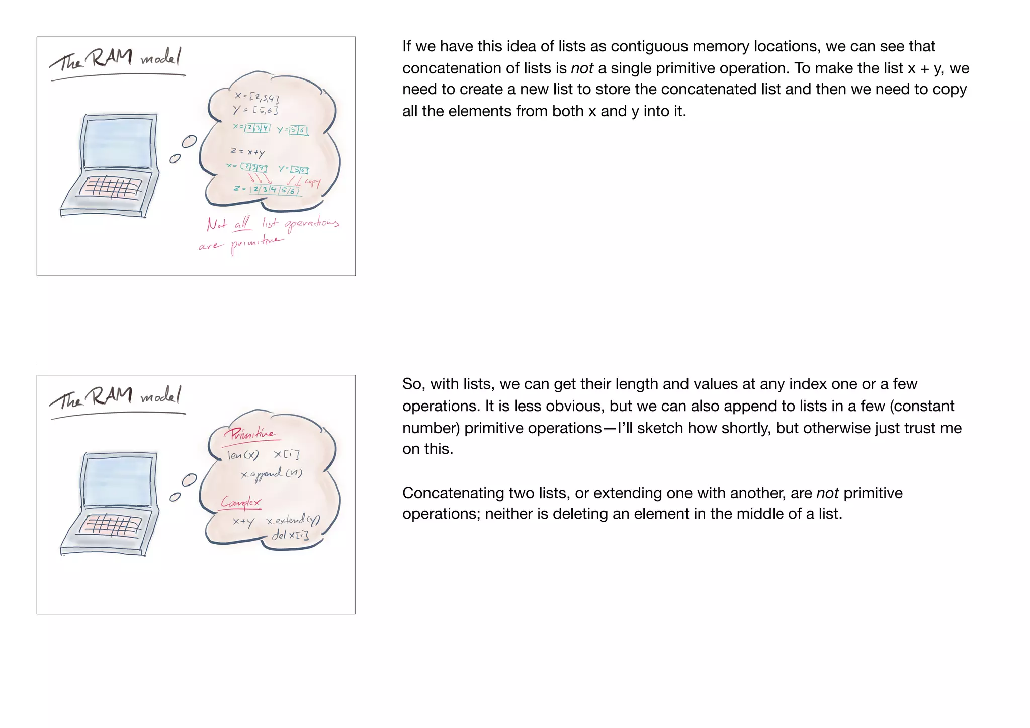
this is a briefer overview about the Big O Notation. Big O Notaion are useful to check the Effeciency of an algorithm and to check its limitation at higher value. with big o notation some examples are also shown about its cases and some functions in c++ are also described.
Data Structures, which is also called as Abstract Data Types (ADT) provide powerful options for programmer. Here is a tutorial which talks about various ADTs - Linked Lists, Stacks, Queues and Sorting Algorithms
Database structure Structures Link list and trees and Recurison complete Adnan abid
Database structure Structures Link list and trees and Recurison complete Database structure Structures Link list and trees and Recurison complete Database structure Structures Link list and trees and Recurison complete Database structure Structures Link list and trees and Recurison complete Database structure Structures Link list and trees and Recurison complete
Database structure Structures Link list and trees and Recurison complete Database structure Structures Link list and trees and Recurison complete Database structure Structures Link list and trees and Recurison complete
Folding Unfolded - Polyglot FP for Fun and Profit - Haskell and Scala - Part 2Philip Schwarz
(download for perfect quality) See aggregation functions defined inductively and implemented using recursion.
Learn how in many cases, tail-recursion and the accumulator trick can be used to avoid stack-overflow errors.
Watch as general aggregation is implemented and see duality theorems capturing the relationship between left folds and right folds.
Through the work of Sergei Winitzki and Richard Bird.
Folding Unfolded - Polyglot FP for Fun and Profit - Haskell and Scala Part 2 ...Philip Schwarz
(download for perfect quality) See aggregation functions defined inductively and implemented using recursion.
Learn how in many cases, tail-recursion and the accumulator trick can be used to avoid stack-overflow errors.
Watch as general aggregation is implemented and see duality theorems capturing the relationship between left folds and right folds.
Through the work of Sergei Winitzki and Richard Bird.
This version corrects the following issues:
slide 32: = reverse --> reverse =
Slide 33: 100_000 -> 1_000_000
It also adds slides 36, 37 and 38
TIME EXECUTION OF DIFFERENT SORTED ALGORITHMSTanya Makkar
what is Algorithm and classification and its complexity
Time Complexity
Time Space trade-off
Asymptotic time complexity of algorithm and its notation
Why do we need to classify running time of algorithm into growth rates?
Big O-h notation and example
Big omega notation and example
Big theta notation and its example
best among the 3 notation
finding complexity f(n) for certain cases
1. Average case
2.Best case
3.Worst case
Searching
Sorting
complexity of Sorting
Conclusion
ADA Unit-1 Algorithmic Foundations Analysis, Design, and Efficiency.pdfRGPV De Bunkers
Title: Algorithmic Foundations: Analysis, Design, and Efficiency
Description:
This PDF document explores the fundamental concepts of algorithms in the subject "Analysis & Design of Algorithm." Delve into the intricate world of algorithmic problem-solving as we cover various topics, including algorithms, designing algorithms, analyzing algorithms, asymptotic notations, heap and heap sort, introduction to the divide and conquer technique, and analysis, design, and comparison of various algorithms based on this technique.
Discover the essence of algorithmic efficiency and learn to evaluate the performance of algorithms using asymptotic notations, such as Big O, Omega, and Theta. Understand the principles of designing algorithms using the divide and conquer approach, which involves breaking complex problems into manageable subproblems and combining their solutions to solve the original problem.
Explore prominent sorting algorithms like merge sort and quick sort, which showcase the power of divide and conquer in tackling real-world challenges. Witness the elegance of Strassen's matrix multiplication, a divide and conquer-based method that optimizes matrix multiplication for large datasets.
This comprehensive PDF is a valuable resource for computer science enthusiasts, students, and professionals seeking to enhance their algorithmic knowledge and design efficient solutions for computational problems. Immerse yourself in the world of algorithms, unravel their intricacies, and master the art of crafting algorithms with optimal performance.
A for loop is probably the most common type of loop in Python. A for loop will select items from any iterable. In Python an iterable is any container (list, tuple, set, dictionary), as well as many other important objects such as generator function, generator expressions, the results of builtin functions such as filter, map, range and many other items.
Similar to Chapter 4 algorithmic efficiency handouts (with notes) (20)
This pdf is about the Schizophrenia.
For more details visit on YouTube; @SELF-EXPLANATORY;
https://www.youtube.com/channel/UCAiarMZDNhe1A3Rnpr_WkzA/videos
Thanks...!
A brief information about the SCOP protein database used in bioinformatics.
The Structural Classification of Proteins (SCOP) database is a comprehensive and authoritative resource for the structural and evolutionary relationships of proteins. It provides a detailed and curated classification of protein structures, grouping them into families, superfamilies, and folds based on their structural and sequence similarities.
(May 29th, 2024) Advancements in Intravital Microscopy- Insights for Preclini...Scintica Instrumentation
Intravital microscopy (IVM) is a powerful tool utilized to study cellular behavior over time and space in vivo. Much of our understanding of cell biology has been accomplished using various in vitro and ex vivo methods; however, these studies do not necessarily reflect the natural dynamics of biological processes. Unlike traditional cell culture or fixed tissue imaging, IVM allows for the ultra-fast high-resolution imaging of cellular processes over time and space and were studied in its natural environment. Real-time visualization of biological processes in the context of an intact organism helps maintain physiological relevance and provide insights into the progression of disease, response to treatments or developmental processes.
In this webinar we give an overview of advanced applications of the IVM system in preclinical research. IVIM technology is a provider of all-in-one intravital microscopy systems and solutions optimized for in vivo imaging of live animal models at sub-micron resolution. The system’s unique features and user-friendly software enables researchers to probe fast dynamic biological processes such as immune cell tracking, cell-cell interaction as well as vascularization and tumor metastasis with exceptional detail. This webinar will also give an overview of IVM being utilized in drug development, offering a view into the intricate interaction between drugs/nanoparticles and tissues in vivo and allows for the evaluation of therapeutic intervention in a variety of tissues and organs. This interdisciplinary collaboration continues to drive the advancements of novel therapeutic strategies.
Professional air quality monitoring systems provide immediate, on-site data for analysis, compliance, and decision-making.
Monitor common gases, weather parameters, particulates.
Observation of Io’s Resurfacing via Plume Deposition Using Ground-based Adapt...Sérgio Sacani
Since volcanic activity was first discovered on Io from Voyager images in 1979, changes
on Io’s surface have been monitored from both spacecraft and ground-based telescopes.
Here, we present the highest spatial resolution images of Io ever obtained from a groundbased telescope. These images, acquired by the SHARK-VIS instrument on the Large
Binocular Telescope, show evidence of a major resurfacing event on Io’s trailing hemisphere. When compared to the most recent spacecraft images, the SHARK-VIS images
show that a plume deposit from a powerful eruption at Pillan Patera has covered part
of the long-lived Pele plume deposit. Although this type of resurfacing event may be common on Io, few have been detected due to the rarity of spacecraft visits and the previously low spatial resolution available from Earth-based telescopes. The SHARK-VIS instrument ushers in a new era of high resolution imaging of Io’s surface using adaptive
optics at visible wavelengths.
Cancer cell metabolism: special Reference to Lactate PathwayAADYARAJPANDEY1
Normal Cell Metabolism:
Cellular respiration describes the series of steps that cells use to break down sugar and other chemicals to get the energy we need to function.
Energy is stored in the bonds of glucose and when glucose is broken down, much of that energy is released.
Cell utilize energy in the form of ATP.
The first step of respiration is called glycolysis. In a series of steps, glycolysis breaks glucose into two smaller molecules - a chemical called pyruvate. A small amount of ATP is formed during this process.
Most healthy cells continue the breakdown in a second process, called the Kreb's cycle. The Kreb's cycle allows cells to “burn” the pyruvates made in glycolysis to get more ATP.
The last step in the breakdown of glucose is called oxidative phosphorylation (Ox-Phos).
It takes place in specialized cell structures called mitochondria. This process produces a large amount of ATP. Importantly, cells need oxygen to complete oxidative phosphorylation.
If a cell completes only glycolysis, only 2 molecules of ATP are made per glucose. However, if the cell completes the entire respiration process (glycolysis - Kreb's - oxidative phosphorylation), about 36 molecules of ATP are created, giving it much more energy to use.
IN CANCER CELL:
Unlike healthy cells that "burn" the entire molecule of sugar to capture a large amount of energy as ATP, cancer cells are wasteful.
Cancer cells only partially break down sugar molecules. They overuse the first step of respiration, glycolysis. They frequently do not complete the second step, oxidative phosphorylation.
This results in only 2 molecules of ATP per each glucose molecule instead of the 36 or so ATPs healthy cells gain. As a result, cancer cells need to use a lot more sugar molecules to get enough energy to survive.
introduction to WARBERG PHENOMENA:
WARBURG EFFECT Usually, cancer cells are highly glycolytic (glucose addiction) and take up more glucose than do normal cells from outside.
Otto Heinrich Warburg (; 8 October 1883 – 1 August 1970) In 1931 was awarded the Nobel Prize in Physiology for his "discovery of the nature and mode of action of the respiratory enzyme.
WARNBURG EFFECT : cancer cells under aerobic (well-oxygenated) conditions to metabolize glucose to lactate (aerobic glycolysis) is known as the Warburg effect. Warburg made the observation that tumor slices consume glucose and secrete lactate at a higher rate than normal tissues.
Introduction:
RNA interference (RNAi) or Post-Transcriptional Gene Silencing (PTGS) is an important biological process for modulating eukaryotic gene expression.
It is highly conserved process of posttranscriptional gene silencing by which double stranded RNA (dsRNA) causes sequence-specific degradation of mRNA sequences.
dsRNA-induced gene silencing (RNAi) is reported in a wide range of eukaryotes ranging from worms, insects, mammals and plants.
This process mediates resistance to both endogenous parasitic and exogenous pathogenic nucleic acids, and regulates the expression of protein-coding genes.
What are small ncRNAs?
micro RNA (miRNA)
short interfering RNA (siRNA)
Properties of small non-coding RNA:
Involved in silencing mRNA transcripts.
Called “small” because they are usually only about 21-24 nucleotides long.
Synthesized by first cutting up longer precursor sequences (like the 61nt one that Lee discovered).
Silence an mRNA by base pairing with some sequence on the mRNA.
Discovery of siRNA?
The first small RNA:
In 1993 Rosalind Lee (Victor Ambros lab) was studying a non- coding gene in C. elegans, lin-4, that was involved in silencing of another gene, lin-14, at the appropriate time in the
development of the worm C. elegans.
Two small transcripts of lin-4 (22nt and 61nt) were found to be complementary to a sequence in the 3' UTR of lin-14.
Because lin-4 encoded no protein, she deduced that it must be these transcripts that are causing the silencing by RNA-RNA interactions.
Types of RNAi ( non coding RNA)
MiRNA
Length (23-25 nt)
Trans acting
Binds with target MRNA in mismatch
Translation inhibition
Si RNA
Length 21 nt.
Cis acting
Bind with target Mrna in perfect complementary sequence
Piwi-RNA
Length ; 25 to 36 nt.
Expressed in Germ Cells
Regulates trnasposomes activity
MECHANISM OF RNAI:
First the double-stranded RNA teams up with a protein complex named Dicer, which cuts the long RNA into short pieces.
Then another protein complex called RISC (RNA-induced silencing complex) discards one of the two RNA strands.
The RISC-docked, single-stranded RNA then pairs with the homologous mRNA and destroys it.
THE RISC COMPLEX:
RISC is large(>500kD) RNA multi- protein Binding complex which triggers MRNA degradation in response to MRNA
Unwinding of double stranded Si RNA by ATP independent Helicase
Active component of RISC is Ago proteins( ENDONUCLEASE) which cleave target MRNA.
DICER: endonuclease (RNase Family III)
Argonaute: Central Component of the RNA-Induced Silencing Complex (RISC)
One strand of the dsRNA produced by Dicer is retained in the RISC complex in association with Argonaute
ARGONAUTE PROTEIN :
1.PAZ(PIWI/Argonaute/ Zwille)- Recognition of target MRNA
2.PIWI (p-element induced wimpy Testis)- breaks Phosphodiester bond of mRNA.)RNAse H activity.
MiRNA:
The Double-stranded RNAs are naturally produced in eukaryotic cells during development, and they have a key role in regulating gene expression .
Comparing Evolved Extractive Text Summary Scores of Bidirectional Encoder Rep...University of Maribor
Slides from:
11th International Conference on Electrical, Electronics and Computer Engineering (IcETRAN), Niš, 3-6 June 2024
Track: Artificial Intelligence
https://www.etran.rs/2024/en/home-english/
What is greenhouse gasses and how many gasses are there to affect the Earth.moosaasad1975
What are greenhouse gasses how they affect the earth and its environment what is the future of the environment and earth how the weather and the climate effects.
1. Chapter 4
Algorithmic Complexity/Efficiency
To think about the complexity of computation, we need a model of reality. As with
everything else in the real world, we cannot handle the full complexity, so we make
some simplifications that enables us to reason about the world.
2. A common model in computer science is the RAM (random access memory)
model. It is the model that we will use.
It shares some commonalities with other models, though not all, so do not think
that the explanation here is unique to the RAM model, but different models can
have slightly different assumptions about what you can do as "primitive"
operations and which you cannot. That is usually the main difference between
them; another is the cost of operations that can vary from model to model.
Common for most the models is an assumption about what you can do with
numbers, especially what you can do with numbers smaller than the input size. The
space it takes to store a number, and the time it takes to operate on it, is not
constant. The number of bits you need to store and manipulate depends on the
size of the number.
Many list operations will also be primitive in the RAM model. Not because the RAM
model knows anything about Python lists—it doesn’t—but because we can
express Python lists in terms of the RAM model (with some assumptions about
how lists are represented).
The RAM has a concept of memory as contiguous "memory words", and a Python
list can thought of as a contiguous sequence of memory words. (Things get a little
bit more complex if lists store something other than numbers, but we don’t care
about that right now). Lists also explicitly store their length, so we can get that
without having to run through the list and count.
In the RAM model we can get what is at any memory location as a primitive
operation and we can store a value at any memory location as a primitive
operation. To get the index of a list, we get the memory location of the list and then
3. If we have this idea of lists as contiguous memory locations, we can see that
concatenation of lists is not a single primitive operation. To make the list x + y, we
need to create a new list to store the concatenated list and then we need to copy
all the elements from both x and y into it.
So, with lists, we can get their length and values at any index one or a few
operations. It is less obvious, but we can also append to lists in a few (constant
number) primitive operations—I’ll sketch how shortly, but otherwise just trust me
on this.
Concatenating two lists, or extending one with another, are not primitive
operations; neither is deleting an element in the middle of a list.
4. You can see that the primitive list operations map to one or perhaps a handful of
primitive operations in a model that just work with memory words, simply by
mapping a list to a sequence of words.
The append operation is—as I said—a bit more complex, but it works because we
have usually allocated a bit more memory than we need for a list, so we have
empty words following the list items, and we can put the appended value there.
This doesn’t always work, because sometimes we run out of this extra memory,
and then we need to do more. We can set it up such that this happens sufficiently
infrequently that appending takes a few primitive operations on average.
Thinking of the lists as contiguous blocks of memory also makes it clear why
concatenating and extending lists are not primitive, but requires a number of
operations proportional to the lengths of the lists.
5. If you delete an element inside the list, you need to copy all the preceding items,
so that is also an operation that requires a number of primitive operations that is
proportional to the number of items copied. (You can delete the last element with a
few operations because you do not need to copy any items in that case).
Assumptions:
• All primitive operations take the
same time
• The cost of complex operations
is the sum of their primitive
operations
When we figure out how much time it takes to solve a particular problem, we
simply count the number of primitive operations the task takes. We do not
distinguish between the types of operations—that would be too hard, trust me, and
wouldn’t necessarily map well to actual hardware.
In all honesty, I am lying when I tell you that there even are such things as complex
operations. There are operations in Python that looks like they are operations at the
same level as getting the value at index i in list x, x[i], but are actually more
complicated. I call such things "complex operations", but the only reason that I
have to distinguish between primitive and complex operations is that a lot is
hidden from you when you ask Python to do such things as concatenate two lists
(or two strings) or when you slice out parts of a list. At the most primitive level, the
computer doesn’t have complex operations. If you had to implement Python based
only one the primitive operations you have there, then you would appreciate that
6. For some operations it isn’t necessarily clear exactly how many primitive
operations we need.
Can we assign to and read from variables in constant time? If we equate variable
names with memory locations, then yes, but otherwise it might be more complex.
When we do an operation such as "x = x + 5" do we count that as "read the value
of x" then "add 5 to it" and finally "put the result in the memory location referred to
as x"? That would be three operations. But hardware might support adding a
constant to a location as a single operation—quite frequently—so "x += 5" might
be faster; only one primitive operation.
Similarly, the number of operations it takes to access or update items at a given
index into a list can vary depending on how we imagine they are done. If the
variable x indicates the start address of the elements in the list (ignoring where we
store the length of the list), then we can get index i by adding i to x: x[0] is memory
address x, x[1] is memory address x + 1, …, x[i] is memory address x + i. Getting
that value could be
1.get x
2.add i
3.read has is at the address x+i
that would be three operations. Most hardware can combine some of them,
though. There are instructions that can take a location and an offset and get the
value in that word as a single instruction. That would be
7. When we have operations that involve moving or looking at more than one memory
word we have a complex operation. These operations typically take time
proportional to how many elements you look at your or you move around.
Extending a list is also a complex operation. We do not (necessarily) need to copy
the vector we modify, but we do need to copy all the elements from the second
vector.
8. When we construct a list from a sequence of values, we have another complex
operation. We need to create the space for the list—this can take time proportional
to the length of the list or constant time, depending on how memory is managed—
and then we need to move all the elements into the list—costing whatever time
that takes.
Appending to a list is actually also a complex operation. We will just treat it as a
primitive one because it can be implemented such that on average it takes a fixed
number of primitive operations to implement. It is actually a bit better than just
saying "on average", it always take a linear number of operations to append n
elements. Such a sequence of append-operations will consist of some cheap and
some expensive operations, but amortised over the n appends we end up with on
the order of n operations.
How this actually works we have to leave for later, but the essence is that lists
allocate a bit more memory than they need and can put new items there. Whenever
it runs out of memory it allocates a block that is twice as large as it was when it ran
out of memory. It turns out that this strategy lets us pretend that appending to a list
always takes a fixed number of primitive operations. We just call it one operation.
9. When we discuss the complexity of an algorithm, we usually discard the cost of
getting the input of passing on the output. We assume that the input is given to us
in a form that we can immediately use, and we assume that the way we leave the
output matches what the next computation needs.
We usually measure the cost of running an algorithm as a function of the input size.
This, by convention, we call n.
It is usually not a problem to see what the size of the input is. If you get a list, it is
the length of the list. If it is a string, it is the length of the string. If it is a graph—like
the connected component algorithm from the previous chapter—then it is the
number of nodes and the number of edges (cities and roads in that example).
One case where it might be a bit strange is when numbers are involved. It takes log
n bits (log base 2) to represent the number n. So if we have a list of n numbers, all
smaller than n, is the input size then n × log n? Of if the input is just a number do
we have n=1 or the log of that number?
This is an issue, but it hardly ever matters. Unless you use numbers larger than
10. To work out the complexity of an algorithm (or, with a positive spin on it, the
efficiency) we count how many operations it takes on input of size n.
Best case?
Average case?
Worst case?
Sometimes, the running time is not just a function of the size of the input but also
what the actual input is. Taking into account all possible input to give a measure of
algorithmic efficiency is impractical, so we use instead consider best, average and
worst-case running times.
11. = n
Counting the actual number of operations is tedious and pointless—it doesn’t
directly translate into running time anyway. We therefore only care about the
"order" of the complexity.
The "Big-Oh of f" class of functions, for some specific function f, are those that f
can dominate after a while if we get to multiply it with a constant.
If g is in O(f) it doesn’t mean that g(n) is smaller than f(n). It is possible that g(n) is
always larger than f(n). But it does mean that we can multiply f with a constant c
such that cf(n) >= g(n) (eventually). The "eventually" means that after some n it is
always the case. It doesn’t mean that cf(n) is always larger than g(n). For some
finite number of points at the beginning of the n axis it can be larger.
12. You get big-Omega by changing which function should dominate which.
If g is in O(f) then f is in Ω(g). (If both, then g is in Θ(f) and f is in Θ(g)).
If you do the arithmetic (for function addition, i.e. (f₁ + f₂)(x) = f₁(x) + f₂(x) and (f · g)
(x) = f(x) × g(x)) it is not hard to show these properties.
The second and third are just special cases of the first, but we use these two more
often than the others.
The second rule tells us that if we have different phases in an algorithm, then we
can add the complexity of those to get the complexity of the algorithm.
The third rule tells us that we really only care about the slowest step of an algorithm
— it dominates all the other steps.
13. The multiplication rules are useful for reasoning about loops. If we do something
that takes constant time at most f(n) times, we have an O(f) running time. Similarly,
if we, f(n) times, do something that takes g(n) times, then we have O(fg). It doesn’t
even have to be exactly f(n) and g(n) times, it suffices that it is O(f) and O(g).
Some complexity classes pop up surprisingly often:
1.Constant time — O(1)
2.logarithmic time — O(log n) — e.g. binary search
3.linear time — O(n) — e.g. linear search
4.log-linear — O(n log n) — e.g. several divide-and-conquer sorting algorithms
5.quadratic time — O(n²) — e.g. simple sorting algorithms
6.cubic time — O(n³) — e.g. straightforward matrix multiplication
7.exponential time — O(2ⁿ) (although it doesn’t have to be base two) — e.g. a lot of
optimisation algorithms. For anything but tiny n this is not usable in practise.
14. Thats it!
Now it is time to do the
exercises to test that
you now understand
algorithmic complexity