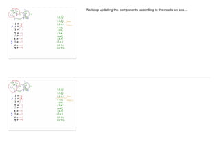
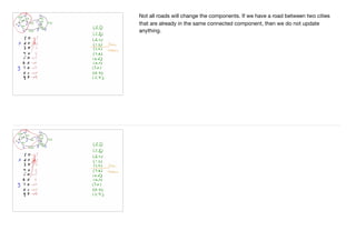
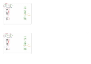
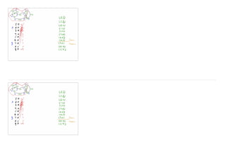
This document provides an introduction and definition of algorithms. It begins by discussing what algorithms are at a high level, noting they are sets of rules or steps to solve specific problems. It then provides a more formal definition, stating an algorithm is a finite sequence of unambiguous steps that solves a specific problem and always terminates. The document discusses the basic building blocks of algorithms, including sequential execution, branching, looping, and variables. It also covers designing algorithms by breaking large problems into smaller subproblems and using preconditions and postconditions. Finally, it provides an example algorithm to determine if two cities are connected on a map and discusses how to prove the correctness of algorithms.

1. Introduction to
Algorithms
What are algorithms?
The topic for this lecture is algorithms, so it is not unreasonable to ask “what is an
algorithm?”; what does “algorithm” mean?

2. https://www.dictionary.com/browse/algorithm
The dictionary definition is “a set of rules to be followed in calculations” with a bit
more fluff around that. So it is something like a recipe to follow if we want to solve
a problem.
Don’t try to figure out what the name means, it is just a reference to Muhammad
ibn Musa al-Khwarizmi, a 9th century mathematician. Algorithm is a latinisation of
al-Khwarizmi and means man from Khwarizmi, similar to how Leonardo da Vinci is
Leonardo from Vinci. There is no deeper meaning to the name.)
al-Khwarizmi wrote a book named “the compendium on calculation by restoring
and balancing” (“al-mukhtasar fi hisab al-jabr wa al-muqabala”), which is where
we have the word algebra from. He didn’t invent algorithms — there are older
known algorithms — we have just named them after him.
That an algorithm is “a set of rules to be followed in calculations” doesn’t quite cut
it. We are not particularly interested in just sets of rules. If we use an algorithm to
solve a problem, we damn well expect it to give us a correct solution!

3. If we shop around some more in dictionaries we also find that the number of
instructions should be finite and unambiguous. We can probably agree that these
are good properties as well.
Combining definitions…
Algorithm (noun):
A finite sequence of unambiguous steps that solves a
specific problem.
So, if we have a specific problem, an algorithm that solves it is
• a finite sequence of steps to take
• these steps are unambiguous — there shouldn’t be any confusion about what
they do (if there is, Murphy's law is guaranteed to be in effect)
• if we follow the steps exactly, we get a solution to the problem.

4. Combining definitions…
Algorithm (noun):
A finite sequence of unambiguous steps that solves a
specific problem.
while True:
print("foo")
When we say we want a finite sequence of steps, we actually require a bit more. It
is possible to have a finite selection of steps that are repeated infinitely often. That
won’t do!
Combining definitions…
Algorithm (noun):
A finite sequence of unambiguous steps that solves a
specific problem.
while True:
print("foo")
We want our algorithms to terminate!
We will not consider a recipe to be an algorithm unless we always get an answer in
a finite number of steps. We say that an algorithm must terminate. Not just on
some input but on all (valid) input. We make no claims about how many steps it
takes to complete an algorithm—it could take nanoseconds or billions of years for
we cares in the definition. We just want to know that eventually we get an answer.
Determining if a given program always terminate is a hard problem. It is impossible
to build an algorithm that does this. Not just hard; it is literally impossible. This
doesn’t mean that we can prove termination in special cases, and we will.
We don’t always want programs to terminate—servers, for example, should run
indefinitely, but those are special cases.

5. Algorithm (noun):
A finite sequence of unambiguous steps that solves a
specific problem.
Cartoon from http://www.sciencecartoonsplus.com/gallery/math/math07.gif
Copied under fair use, see https://rationalwiki.org/wiki/File:Math07.gif
Combining definitions…
Steps should be specific enough that we know we can follow them.
Feynman’s problem solving algorithm:
Write down the problem.
Think very hard.
Write down the solution.
If we leave some steps sufficiently vague not only do we leave room for errors, we
have a recipe that other’s might not be possible to follow. We need enough detail
that it is clear what must be done in each step. We usually stop short of reaching
them level of detail a computer needs to carry out the step. That is what we do
when we implement an algorithm.
Whether steps are unambiguous is a bit subjective…
Combining definitions…
Algorithm (noun):
A finite sequence of unambiguous steps that solves a
specific problem.
Given that we have a finite description of a problem—that will actually only perform
a finite number of steps on any (valid) input—and that the description gives us an
unambiguous description of what to do, we know that we always get an answer in
finite time. It would be a bonus if we always knew that the answer was actually
correct!
In this class, we will make that part of the definition. We say that an algorithm is
correct if it always gives us a correct solution, and correctness is something we
need to prove when we develop a new algorithm. Correctness isn’t always part of
the definition. Sometimes we can live with an algorithm being correct with high
probability. In this class, though, we want correctness.

6. Building-blocks in
Programming and in
Algorithms
Before we discuss how we ensure the properties we want recipes to have to be
considered algorithms, and how we approach designing algorithms to satisfy them,
let us consider the building blocks of algorithms and compare them to the
programming constructs we are familiar with.
Sequential
Branching
Looping
There are no substantial difference in the flow of operations. When we write
programs, we might have high-level operations available for designing programs,
but at the most fundamental level, we can do one operation after another, repeat a
series of operations a number of times, or choose two different paths along a
program based our program’s state. (At a more primitive level, we have conditional
and un-conditional jumps between operations, but the nature of these
constructions make it worth treating them as three different control-flow
constructions).

7. Sequential execution
In an algorithm we can specify an order of operations where one step always goes
before another. This is no different from programs where one statement goes
before another. Algorithmic step are usually at a much higher level of abstraction,
but otherwise there is no difference between sequential execution of a program
and an algorithm.
Variables (program state)
Just as for programs, we have a concept of “state” in an algorithm. In a program,
the state is is determined by which values our variables refer to and the state of
these values. This is no different in an algorithm.
The values we manipulate in a program are restricted in nature based on their type;
a list is always a sequence but it can be modified, a tuple is also a sequence but it
cannot be modified, for example. In an algorithm we often have stronger
requirements on the program state than is handled by the type information in a
program, so-called invariants that we must ensure are always satisfied—more on
this later.

8. Branching
There are no surprises when it comes to branching either; we have the same
operations in an algorithm as we have for a program. Again, an algorithm often
condition on more abstract properties of data than what we use in an if-statement,
but otherwise algorithms are no different from programs (and more complex if-
statements can readily be implemented using predicate functions).
Looping
Yeah, the difference between loops in programs and in algorithms are tiny as well.
Loops are really all the same, but there are some benefits to splitting them into two
categories: those loops that are over a fixed and finite sequence of elements and
those loops that continue until a predicate is false. In Python, we have for- and
while-loops to express which of the types of loops we are working with.
You are not guaranteed that a for-loop is actually iterating over a finite set of
elements in Python, though. The two loop constructions differ in their syntax but a
for-loop is syntactic-sugar for a while-loop. Just because you use a for-loop you
are not guaranteed to loop over a finite sequence. For all our uses of for-loops,
however, we will loop over a finite sequence (and it requires either substantial
carelessness or Python constructions we will not see in this class to change this).

9. Designing algorithms:
Breaking down problems
to smaller parts
Levelsofdetails
They key steps in designing an algorithm is to break large tasks—which we may
not know how to achieve—into sub-steps that each solve part of the problem and
when combined achieve the larger task.
We usually cycle between asking "what do we want to achieve?" and "how do we
achieve this?". We identify what we need the algorithm to do, for example,
compute a phylogenetic tree from an alignment of DNA sequences. That is what
we want to achieve. So how do we achieve it? Well, we can for example break this
task into two sub-tasks: can we calculate a matrix containing all pair-wise
distances between the sequences, and can we compute a tree given such a
matrix? We can reduce the "Infer a tree" task into these two steps; each solve
parts of the problem and if we execute the steps "Calculate distances" and
"Construct tree from matrix", one after another, we have solved the "Infer tree"
problem.

10. Levelsofdetails
You do not, strictly speaking, have to make each task completely independent of
other tasks, but you will want to as a general rule. If you make the tasks
independent, then you can solve any single task without worrying about how your
solution affects the rest of your algorithm.
If we want to solve sub-problems independently, and still guarantee that they will
work when we combine them, we need to be very precise in what each task needs
to do, what it expects of its input, and what it promises about its output.
Levelsofdetails
Pre-condition Post-condition
Pre-condition Post-/Pre-condition
Post-condition
Post-condition
Pre-condition
Post-/Pre-condition
You do not, strictly speaking, have to make each task completely independent of
other tasks, but you will want to as a general rule. If you make the tasks
independent, then you can solve any single task without worrying about how your
solution affects the rest of your algorithm.
If we want to solve sub-problems independently, and still guarantee that they will
work when we combine them, we need to be very precise in what each task needs
to do, what it expects of its input, and what it promises about its output. We call
the demands on the input "preconditions" and the promises about the output
"postconditions".
Regardless of how you perform a task, you can assume that its preconditions are
satisfied, and you need to ensure that its postconditions are satisfied—other tasks
later in the algorithm will depend on it.

11. If we have different paths between two tasks, because we have some conditional
execution, then we have pre- and post-conditions that should be valid for all the
paths.
The pre-condition before the branch, together with the result of the branch-
condition (which can be true or false), should guarantee the pre-conditions of the
different branches, and the post-conditions of all branches should guarantee the
pre-conditions of the point where the branches merge again.

12. In a loop, there are a lot of pre- and post-conditions in play. There are pre-
conditions before we test the loop-condition and before we execute the first step in
the loop-body. There are post-conditions at the end of the loop-body and post-
conditions for when we leave the loop.
The concept "loop invariant" puts restrictions on all these conditions.
Informally, people will say that a loop invariant should always be true inside a loop,
but this isn’t strictly true. It can be violated at any point inside the loop body; it just
needs to be true before and after executing the loop body. The loop invariant work
with the conditions shown in the figure.
We require that the invariant is true before we even test the loop-condition. This
guarantees that the invariant is true whenever we make this check, regardless of
whether it is when we first reach the loop or when we return to the test after
executing the loop body.

13. If the loop-condition is true and the invariant is true, then that should guarantee
that the pre-conditions for the first step in the loop body are true.
Whenever we finish the loop body, the invariant must also be true. This means that
the post-conditions of the last step in the loop body must guarantee the invariant.
After the last step inside the loop body, the loop condition can be both true and
false (if it is always true we will never leave the loop); we do not require that it is
true from the post-condition of the last statement—only that the invariant must be
true.
It is because the invariant must be true before and after we enter the loop body
that we say that it must always be true for a loop—the language is a bit imprecise
but what we mean is that the invariant fits the pre- and post-conditions of the loop
body in this particular way.
When we leave the loop, the loop-condition will be true—otherwise we wouldn’t
leave the loop—and we require that the invariant is also true. These two conditions,
combined, can be seen as the post-condition of the entire loop and they should
guarantee the pre-condition of the first statement after the loop.

14. Example: are cities A
and B connected?
Consider a map — I know I am not earning any art-points here, but I do my best.
The map includes roads between cities and we are interested in knowing if it is
possible to get from city A to city B by road.
There are no cities on earth that you cannot reach from any other, but you cannot
go by road between all pairs of cities. It is a bit of a made up problem, but it is not
unrealistic (and it does pop in many applications where we are interested in
connections between items that are not cities).

15. The actual map doesn’t matter. Only the connections between cities that the
connect pairs of cities.
We can number the cities, so we can refer to them without pointing at the map.

16. And we can represent all the roads by the pair of cities they connect. We consider
(a,b) and (b,a) the same; we do not care about the order.
A structure that only consists of nodes and direct connections between them is
usually called a graph.
We have simplified our data to something that is easier to give to the computer and
perhaps also easier to manipulate in a program.
We can also change the question from "are A and B connected?" to "are A and B
in the same connected component?"
A connected component is a set of graph nodes where you can get from any one
node to all the others. We will derive an algorithm that maps each node to a
connected component; once we have this map, we can decide if A and B are
connected by checking if they are in the same component.

17. We will represent the connected components by a "canonical representative": the
city with the smallest number in the component. We will have each city point to the
representative of its connected component.
We will iterate through the roads and we will have the following invariant:
All cities know their connected component assuming that the graph only had
the roads we have seen so far.
Before we start the loop, each city must point to itself (all components are
singletons if there are no connections).
After each loop-iteration we must have updated the components according to the
new road.
When we see a new road, we have to connect two components. Since we
represent components by the smallest index in them, we need to make all the
cities in both components point to the smallest index in the two components. (Do
not worry about the details of how to do this for now; it suffices to know that this is
what we must do).

18. We keep updating the components according to the roads we see…

19. Not all roads will change the components. If we have a road between two cities
that are already in the same connected component, then we do not update
anything.

22. Once we are done scanning through all the roads, we can simply ask if city A —
index 2 — is in the same component as city B — index 7 — and we see that they
are.

23. Intermezzo
• How would you represent the components in Python?
• How would you formalise the loop invariant to take into
account the representation of the components?
Intermezzo
• Run the algorithm on these two graphs:

24. Correctness
How do we prove
correctness?
• We prove that all pre- and post-conditions are satisfied
through the steps in the algorithm.
• We prove that the post-condition of the last step implies
that the overall problem is solved.
• Correctness is just a special case of post-conditions
There isn’t anything special about the post-condition of the entire algorithm and
any other post-condition. If the post-condition of the algorithm is what we want it
to do, then proving correctness is just an application of proving that post-
conditions are met when pre-conditions are met (for the algorithm, this is
restrictions on the allowed input).

25. Termination
Termination functions:
To ensure that our algorithm
terminations, we add a "termination"
function to each loop.
This is a count-down that should
go down each time we execute the
body of the loop.
An algorithm will terminate if all loops in it terminates. So, we can deal with each
loop at a time. For a loop, we can associate a termination function. This is just a
mapping from the program’s state to a number that is guaranteed to decrease with
each iteration of of the loop body and that will eventually reach zero.
It is possible to define functions that decrease in each loop iteration but never
reaches zero. You can get asymptotically closer to zero in each iteration. In such
cases, we need to be a bit careful with defining the termination function such that it
will eventually go below zero. Generally, though, it is relatively easy to come up
with a termination function that will be zero when the loop-condition is false and
that will decrease in each iteration.

26. For the connectivity problem, the termination function is particularly simple: we use
the number of roads that are left to process.
With the for-loops we have seen, we always iterate over a finite sequence of
elements, so there we can always use the number of items that remain in the
sequence.
Get the binary representation of a number n
Termination function:
t(n) = n
We extract the bits in n in reverse order. We get the least significant bit using
modulus and add that to a list, reverse_bits. When we are done with the loop, we
reverse this list.
The termination function is simply n.
When it is zero, the loop condition is false, and we leave the loop.
In each iteration, we decrease n — we divide it by two.

27. Thats it!
Now it is time to do the
exercises to test that
you now know how to
construct algorithms