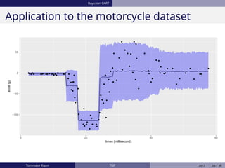
꧁❤ Greater Noida Call Girls Delhi ❤꧂ 9711199171 ☎️ Hard And Sexy Vip Call
Bayesian regression models and treed Gaussian process models
1. Bayesian regression models and treed
Gaussian process models
Tommaso Rigon
22-03-2017
Tommaso Rigon TGP 2017 1 / 36
2. A general regression problem
Let (xi, yi), for i = 1, . . . , n, denotes the collection of a set covariates with
its response variable, respectively. Suppose that
yi | xi
ind
∼ f(yi | xi),
independently for i = 1, . . . , n according to some unknown distribution
function f(yi | xi), with yi ∈ R.
Examples
Linear regression: yi = xT
i β + i, with i ∼ N(0, σ2
);
Heterschedastic errors: yi = xT
i β + i(xi), with i(xi) ∼ N(0, σ2
(xi))
Mean regression: yi = g(xi) + i, for some unknown function g, for
instance having the form g(xi) = h(xi)T
β.
Tommaso Rigon TGP 2017 2 / 36
4. Desiderata
We are looking for a regression model that:
provides a flexible estimate of the mean process (e.g. not linear);
adaptively quantify the uncertainty of the process as the covariates vary
(e.g. not homoschedastic);
can be easily extended to the multivariate setting xi = (xi1, . . . , xip)T
;
is computationally feasible for large n or large p;
has a reasonable interpretation and therefore
can incorporate prior information, if available (e.g. Bayesian).
Tommaso Rigon TGP 2017 4 / 36
5. Bayesian methods for adaptive regression
Bayesian regression model includes
Linear models. Bayesian linear model, Bayesian lasso, Bayesian
elastic-net.
Basis expansion models. e.g. Bayesian splines (regression, penalized
and smoothing splines), Bayesian MARS, wavelets and Gaussian
processes.
Hard partitioning models. e.g. Bayesian CART, Bayesian additive
regression trees (BART), treed Gaussian processes.
Soft partitioning models. e.g. Bayesian mixture of experts, dependent
Dirichlet process, logit stick-breaking process.
Machine learning methods. e.g. support vector machine, Bayesian
neural networks.
Tommaso Rigon TGP 2017 5 / 36
6. Bayesian linear regression
Bayesian linear regression
Regression model prior distribution
Independently for i = 1, . . . , n we let
yi | xi, β, σ2
∼ N(xT
i β, σ2
), β ∼ Np(b, B), σ−2
∼ Gamma(aσ, bσ).
Full conditionals
Let y = (y1, . . . , yn) and X is the design matrix including all the xi, then
the Gibbs sampling alternates between
β | − ∼ Np(˜b, ˜B), ˜b = ˜B B−1
b +
1
σ2
XT
y , ˜B = B−1
+
1
σ2
XT
X
−1
,
and
σ−2
| − ∼ Gamma(˜aσ,˜bσ), ˜aσ = aσ +
n
2
, bσ = bσ +
1
2
(y − Xβ)T
(y − Xβ).
Tommaso Rigon TGP 2017 6 / 36
7. Bayesian linear regression
Bayesian regression with basis expansions
Weighted sum of basis functions
The linear model can be easily extended to
yi | h(xi), β, σ2
∼ N(h(xi)T
β, σ2
), β ∼ NM (b, B), σ−2
∼ Gamma(aσ, bσ).
where the vector h(xi) = (h1(xi), . . . , hM (xi))T
is a prespecified set of
basis functions, such that hm(·) : Rp
→ R, for m = 1, . . . , M.
Basis expansion when p = 1
Possibile choices for the specified basis are
Polynomial basis expansion: h(xi) = (xi, x2
i , . . . , xM
i )T
.
Splines basis (regression splines, penalized splines, smoothing splines).
Wavelets.
Gaussian radial basis functions.
Tommaso Rigon TGP 2017 7 / 36
9. Bayesian linear regression
A limitation of Bayesian P-splines
Posterior variance of the linear predictor
Suppose σ2
is treated as known and let H be the design matrix induced by
h(xi). Then, the posterior variance of ηi = h(xi)T
β is
Var(ηi | y) = h(xi)T ˜Bh(xi), with ˜B = B−1
+
1
σ2
HT
H
−1
.
Thus, the posterior variability is not constant over xi, but it does not
depend on the response, being obtained as a function of H, B, and σ2
.
But σ2
is indeed unknown...
Even if we put a prior on σ2
, the posterior variance will indeed depend on
the data, but only through σ2
, which will control the global variability and
will not capture local variability.
Tommaso Rigon TGP 2017 9 / 36
10. Gaussian Processes
Gaussian processes
Definition (Rasmussen and Williams, 2006)
A Gaussian process f(x), or f for short, is a stochastic process defined on
X = Rp
such that all the finite-dimensional distribution have joint
Gaussian distribution.
A Gaussian process is completely specified by its mean function
m(x) = E(f(x)), ∀x ∈ X,
and the covariance function
k(x, x ) = Cov(f(x), f(x )), ∀x, x ∈ X.
We will write
f ∼ GP(m(x), k(x, x )).
Tommaso Rigon TGP 2017 10 / 36
11. Gaussian Processes
Gaussian processes
Finite dimensional distributions
By definition, for each finite collection of points x = (x1, . . . , xn) all in X we
have that the vector f(x) = (f(x1), . . . , f(xn)) is distributed according to
f(x) ∼ Nn(m(x), K(x, x)),
where m(x) is the n-dimensional mean vector generated by the mean
function and K(x, x) is a n × n covariance matrix generated by k(·, ·) by
setting [K(x, x)]ij = k(xi, xj), for i, j = 1, . . . , n.
Notation
Let x and x be two collections of points in X and let f(x) and f(x ) be the
associated random variables. We let
Cov (f(x), f(x )) = K(x, x ).
Tommaso Rigon TGP 2017 11 / 36
12. Gaussian Processes
Covariance functions
Positive semi-definite functions
For k(·, ·) to be a valid covariance function it has to be a symmetric
positive semi-definite function, that is
k(x, x ) = k(x , x), ∀x, x ∈ X
and for any choice of n, α ∈ Rn
, and for any x = (x1, . . . , xn), it should hold
n
i=1
n
j=1
αiαjk(xi, xj) = αT
K(x, x)α ≥ 0.
Tommaso Rigon TGP 2017 12 / 36
13. Gaussian Processes
Covariance functions
Stationarity
A covariance function k(·, ·) is called stationary if is invariant under any
arbitrary translation t ∈ X, so that
k(x + t, x + t) = k(x, x ), ∀x, x ∈ X,
that is, it is a function of x − x only. A Gaussian process with constant
mean function is strictly stationary if its covariance function is stationary.
Isotropy
A stationary covariance function is called isotropic if it is a function only of
the euclidean distance between x and x , that is
k(x, x ) = k(r), r = ||x − x ||, ∀x, x ∈ X.
Tommaso Rigon TGP 2017 13 / 36
14. Gaussian Processes
Examples of covariance functions
Squared exponential
The squared exponential covariance function has the form
kSE(r) = τ2
exp −
r2
2l2
, τ, l > 0.
Although such a covariance function makes the process very smooth, it is
the most widely-used kernel within the kernel machines field.
Matern class of covariance functions
kMat(r) = τ2 21−ν
Γ(ν)
√
2νr
l
ν
Kν
√
2νr
l
,
with positive parameters ν and l, where Kν is a modified Bessel function.
For ν → ∞ the squared exponential is recovered.
Tommaso Rigon TGP 2017 14 / 36
15. Gaussian Processes
Relationship with other methods
Bayesian linear regression
A Bayesian linear model with Gaussian parameters is a degenerate GP,
having
m(x) = h(x)T
b, k(x, x ) = h(x)T
Bh(x).
A GP is said non degenerate if its covariance function is positive definite.
Smoothing splines (Wahba, 1978)
Smoothing splines can be recasted as a regression with a partially proper
GP prior with a specific covariance matrix.
SVM and neural networks
Further connection with Support Vector Machine and Bayesian neural
networks can be estabilished (Neal 1996, Rasmussen and WIlliams 2006).
Tommaso Rigon TGP 2017 15 / 36
16. Gaussian Processes
A naive Bayesian model via GPs
We assume that the response y depends on multivariate covariates x
through the following functional specification
y(x) = f(x) + (x), ∀x ∈ X,
where f(x) represents the signal and (x) the noise.
Despite the functional specification, we can observe only a finite number
values (xi, yi). Assuming, additionally, that ∼ GP(0, k (x, x )) with
k (x, x ) = σ2
I(x = x ), we obtain
yi | f(xi), σ2 ind
∼ N(f(xi), σ2
), i = 1, . . . , n,
independently. The elicitation is complete by specifying a functional prior
f ∼ GP(0, k(x, x )) and an inverse gamma for σ2
as before.
Tommaso Rigon TGP 2017 16 / 36
17. Gaussian Processes
Posterior inference via Gibbs sampling
Full conditionals (kriging equations)
The Gibbs sampling alternates between
f(x) | y, σ2
∼ Nn( ˜m(x), ˜K(x, x)), and σ−2
| y, f(x) ∼ Gamma(˜aσ,˜bσ),
where
˜m(x) = K(x, x)(K(x, x) + σ2
In)−1
y =
1
σ2
˜K(x, x)y
and
˜K(x, x)) = K(x, x)−1
+
1
σ2
In
−1
= K(x, x) − K(x, x)(K(x, x) + σ2
In)−1
K(x, x)
Tommaso Rigon TGP 2017 17 / 36
18. Gaussian Processes
A more complete specification
Incorporating basis expansions (Blight and Ott, 1975, O’Hagan, 1978)
We assume that
y(x) = h(x)T
β + f(x) + (x), ∀x ∈ X,
where h(x)T
β and f(x) represents the signals and (x) the noise.
Moreover, let f(x) ∼ GP(0, τ2
k∗
(x, x | l)), where k∗
(x, x | l) is a correlation
function, and ∼ GP(0, k (x, x | g)) with k (x, x | g) = gτ2
I(x = x ), so that
y(x) | β, τ2
, g ∼ GP h(x)T
β, τ2
k(x, x | g, l) .
where k(x, x | g, l) = k∗
(x, x | l) + k (x, x | g). Finally, we let
β | τ2
∼ NM (b, τ2
B), τ−2
∼ Gamma(aτ , bτ ).
Tommaso Rigon TGP 2017 18 / 36
19. Gaussian Processes
Some difficulties
Covariance parameters (g, l)
The parameters (g, l) play a crucial roles in fitting a GPs but their prior
elicitation is more delicate. Gramacy and Lee (2008) propose:
p(g, l) = p(g)p(l) = p(g)
1
2
Gamma(l | 1, 20) +
1
2
Gamma(l | 10, 10) ,
with p(g) = Exp(g | ag).
Metropolis-Hastings within Gibbs for (g, l)
Analytically integrating out β and τ2
gives a marginal posterior for
K(x, x | g, l) (Berger et al., 2001), that can be used to obtain efficient MH
draws.
Tommaso Rigon TGP 2017 19 / 36
21. Gaussian Processes
Application to the motorcycle dataset
−100
0
0 20 40 60
times (millisecond)
accel(g)
Tommaso Rigon TGP 2017 21 / 36
22. Gaussian Processes
Brief summary about Gaussian Processes
Advantages
GPs are a powerful tool for nonparametric regression.
GPs are conceptually straightforward and can easily accomodate prior
knowledge.
Uncertainty quantification, e.g. posterior credible intervals, can be easily
taken into account.
Disadvantages
GP models are usually “stationary”, meaning that the same covariance
matrix is used throughout X, which may be a strong assumption.
Moreover, non stationary models are often computationally intractable.
Although some fast approximations exist, fitting a GP usually require the
inversion of n × n matrixes, which has a computing time of O(n3
).
Tommaso Rigon TGP 2017 22 / 36
23. Bayesian CART
Classification and Regression Trees (CART)
Regression trees (Breiman et al. 1984)
CART models are a regression method that recursively partition the
predictor space into subsets, usually through a greedy algorithm, so that
the distribution of y is more and more homogeneous.
...and related methods
Modifications and extensions of CART (e.g. MARS, random forest,
AdaBoosting and gradient boosting), are perhaps one of the most widely
used tool for regression in the machine learning community.
Bayesian CART (Chipman et al. 1998, Denison et al. 1998)
Bayesian modifications of CART were later proposed, introducing a prior
distribution on the partition of the covariates.
Tommaso Rigon TGP 2017 23 / 36
24. Bayesian CART
Bayesian CART model
A binary tree T subdivides X into S non-overlapping regions {R1, . . . , RS},
so that X =
S
s=1 Rs. This is obtained recursively, splitting at each step a
previously obtained region into sub-regions. Each region Rs contains data
(Xs, ys), comprising a total of ns observations, for s = 1, . . . , S.
Conditionally to the tree structure, the CART model assumes independent
observations among regions and observations, that is
yis | θ, T
ind
∼ N(yis | µs, σ2
s ), i = 1 . . . , ns, s = 1, . . . , S.
Prior distribution for θ = (µ, σ2
) are given conditionally to T , i.e. following
the standard Gaussian - inverse gamma specification.
Tommaso Rigon TGP 2017 24 / 36
25. Bayesian CART
An example of tree partitioning
x1 <> 24.2
x1 <> 13.8
1e−04
20 obs
1 x1 <> 17.6
0.0074
11 obs
2
0.0033
15 obs
3
x1 <> 38
0.0724
28 obs
4
0.0053
20 obs
5
A tree of height=4, log(p)=107.594
Tommaso Rigon TGP 2017 25 / 36
26. Bayesian CART
A tree prior for T
An implicitely defined tree prior (Chipman et al., 1998)
The prior stochastic process for T is described here in a recursive manner.
Begin by setting T to be the trivial tree with a single region R = X.
Each terminal region Rs splits in Rs1 ∪ Rs2 with probability a(1 + qRs )−b
,
where qRs
is the depth of Rs, i.e. the number of splits above Rs. The
split rule consists is chosing randomly and uniformly among the values
of the observed covariates X.
If new regions are created, repeat step 2 until the process stops.
Tommaso Rigon TGP 2017 26 / 36
27. Bayesian CART
Prior distribution: # of terminal nodes0.00.20.4
alpha=0.5 and beta=0.5
Number of terminal nodes
Probability
1 3 5 7 9 11 13 15 17 19 21
0.000.040.08
alpha=0.95 and beta=0.5
Number of terminal nodes
Probability
1 6 12 19 26 33 40 47 54 61 78
0.000.100.20
alpha=0.95 and beta=1
Number of terminal nodes
Probability
1 3 5 7 9 11 13 15 17 19
0.00.20.4
alpha=0.95 and beta=1.5
Number of terminal nodes
Probability
1 2 3 4 5 6 7 8 9 10 12 15
Tommaso Rigon TGP 2017 27 / 36
28. Bayesian CART
Posterior inference
A RJ-MCMC algorithm (Chipman et al. 1998)
A reversible jump Metropolis-Hastings algorithm is used for posterior
computation, which involves the following reversible steps
GROW. Randomly pick a terminal node and split it into two new ones.
PRUNE. Randomly pick a parent of two terminal nodes and turn it into a
terminal node.
CHANGE. Randomly pick an internal node and randomly reassign it a
splitting rule.
SWAP. Randomly pick a parent-child pair and swap their splitting rule.
Tommaso Rigon TGP 2017 28 / 36
29. Bayesian CART
Application to the motorcycle dataset
−100
−50
0
50
0 20 40 60
times (millisecond)
accel(g)
Tommaso Rigon TGP 2017 29 / 36
30. Bayesian CART
Limitations and extensions
Potential limitations
Slow mixing. The entire MCMC procedure get easily stuck into some
local mode and therefore it is recommended to restart the chain several
times to explore different solutions.
Difficulties in capturing smooth or even linear behaviour via piecewise
constant functions.
Extensions
A treed Bayesian linear model was proposed by Chipman et al. (2002), in
which at each terminal node is assumed to be a linear model.
An additive Bayesian model based on Bayesian CART, called BART, was
proposed by Chipman et al. (2010), which mostly solves the issues
underlined above.
Tommaso Rigon TGP 2017 30 / 36
31. Treed Gaussian Process Model
Treed Gaussian Processes
The conditional model (Gramacy and Lee 2008)
Conditionally to a tree structure T , the treed Gaussian process model
assumes
y(x) = h(x)T
βs + fs(x) + s(x), ∀x ∈ Rs, s = 1, . . . , S,
fs(x)
ind
∼ GP(0, τ2
s k∗
(x, x | ls)), s
ind
∼ GP(0, k (x, x | gs)),
where h(x) = (1, x)T
, k∗
(x, x | ls) and k (x, x | gs) = gsτ2
s I(x = x ) are
correlations functions. Moreover, we have
βs | bs, τ2
s , κ2
s, B
ind
∼ NM (bs, τ2
s κ2
sB).
For the tree structure T , the same prior as in Chipman et al. (1998) is
assumed.
Tommaso Rigon TGP 2017 31 / 36
32. Treed Gaussian Process Model
More on prior elicitation
Hyperpriors...
The model elicitation is completed by assuming
bs
i.i.d
∼ NM (b0, B0), B−1
s
i.i.d
∼ W((ρV )−1
, ρ),
τ−2
s
i.i.d
∼ Gamma(aτ , bτ ), κ−2
s
i.i.d
∼ Gamma(aκ, bκ),
where W represent the Wishart distribution. Mixture priors for the
parameters (gs, ls), for s = 1, . . . , S are also assumed, similarly to what
discussed before.
...and hyperparameters
Default values for the hyperparameters of the tree are suggested by the
authors and setted equal to a = .5 and b = 2.
Tommaso Rigon TGP 2017 32 / 36
33. Treed Gaussian Process Model
Posterior inference
Posterior inference resembles the RJ-MCMC of Chipman et al. (1998),
with an additional operation called ROTATE, which should improve the
mixing, by providing a more dynamic set of candidate nodes for pruning.
Conditionally to the tree structure, full conditional inference for most of
the involved parameters is available, independently for each region, so
that a Gibbs sampler can be setted up.
Metropolis-Hastings within Gibbs steps are required for each pair (gs, ls).
The usual predictive (kriging) equations are also available, conditionally
to each region Rs.
Tommaso Rigon TGP 2017 33 / 36
34. Treed Gaussian Process Model
Implementation and software
Software (Gramacy 2007)
An R package called tgp was made available, which can handle all the
models discussed so far and even more, for instance allowing for
parallelization of the MCMC chain.
The tree GP model was coded in a mixture of C and C++, then wrapped by
R commands. Centering and rescaling the input is reccommended by the
authors, so that defualt Metropolis-Hastings proposal distributions can be
used.
Tommaso Rigon TGP 2017 34 / 36
35. Treed Gaussian Process Model
Application to the motorcycle dataset
−100
0
0 20 40 60
times (millisecond)
accel(g)
Tommaso Rigon TGP 2017 35 / 36
36. Treed Gaussian Process Model
Discussion and possible extensions
Limiting linear models (Gramacy and Lee 2008)
In some cases a GP may not be needed within a partition, and a much
simpler model, such as the linear model, may suffice. Linear models can
be viewed as a particular case of a GP, and a model-switching prior
distribution for the hyperparameters (g, l) would allow the practical
implementation.
Treed GP for classification (Broderick and Gramacy, 2010)
Treed Gaussian processes could also be used when y ∈ {0, 1}, therefore
assuming a flexible representation for P(yi = 1 | xi).
A more complex input space X (Broderick and Gramacy, 2011)
So far we have assumed that X = Rp
, but more complex input space could
be of interest, for instance when some of the inputs are categorical.
Tommaso Rigon TGP 2017 36 / 36