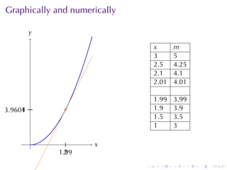
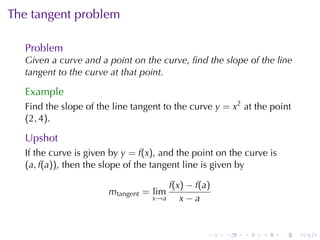
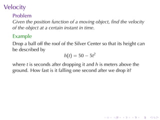
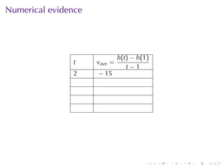
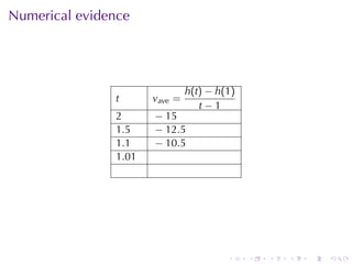
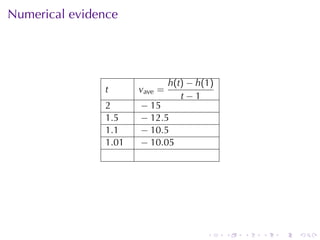
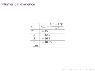
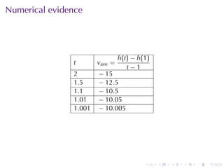
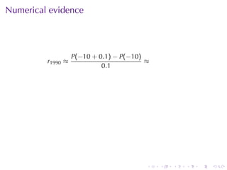
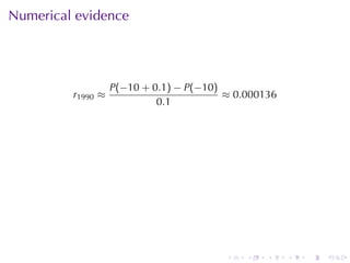
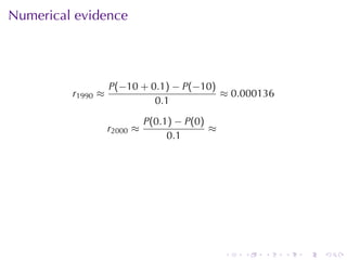
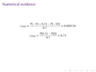
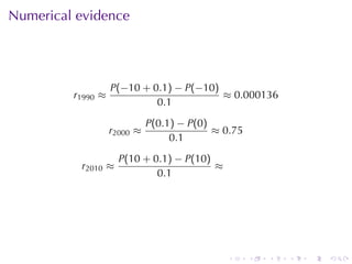
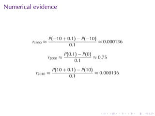
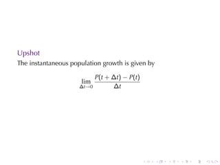
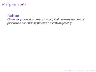
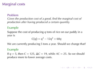
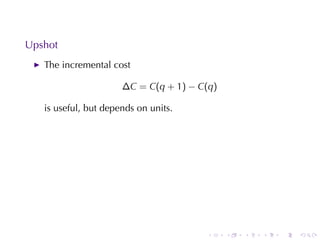
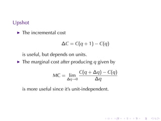
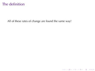
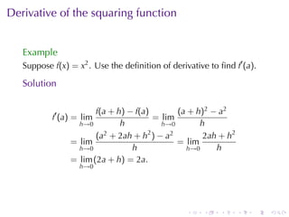
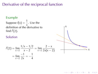
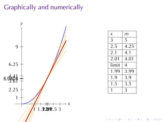
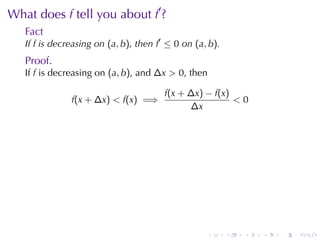
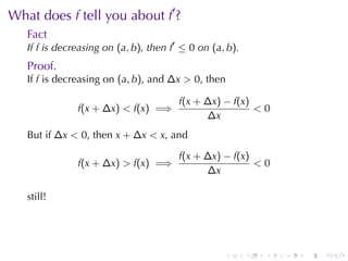
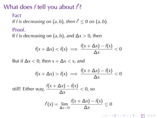
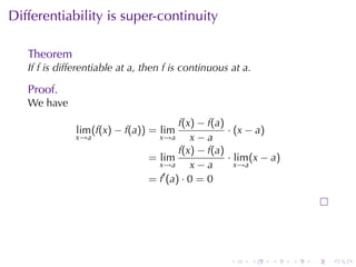
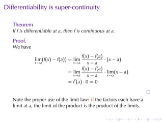
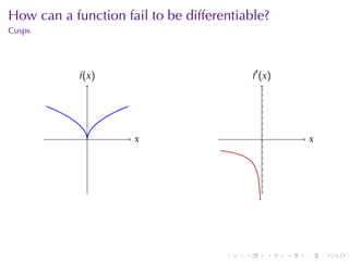
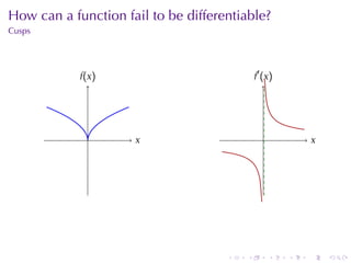
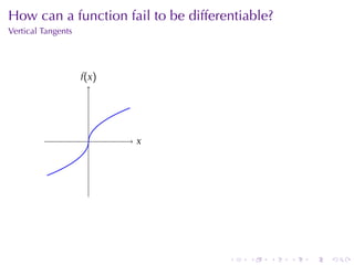
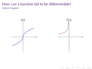
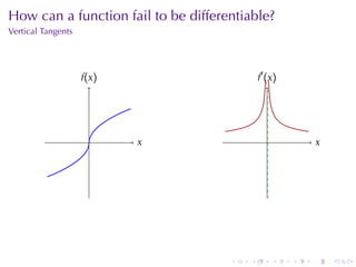
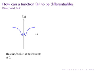
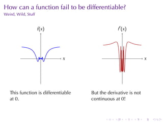
. . . . . .
Section	2.1
The	Derivative	and	Rates	of	Change
V63.0121.034, Calculus	I
September	23, 2009
Announcements
WebAssignments	due	Monday. Email	me	if	you	need	an
extension	for	Yom	Kippur.
. . . . . .
Regarding	WebAssign
We	feel	your	pain
. . . . . .
Explanations
From	the	syllabus:
Graders	will	be	expecting	you	to	express	your	ideas
clearly, legibly, and	completely, often	requiring
complete	English	sentences	rather	than	merely	just	a
long	string	of	equations	or	unconnected	mathematical
expressions. This	means	you	could	lose	points	for
unexplained	answers.
. . . . . .
Rubric
Points Description	of	Work
3 Work	 is	 completely	 accurate	 and	 essentially	 perfect.
Work	is	thoroughly	developed, neat, and	easy	to	read.
Complete	sentences	are	used.
2 Work	 is	 good, but	 incompletely	 developed, hard	 to
read, unexplained, or	 jumbled. Answers	 which	 are
not	explained, even	if	correct, will	generally	receive	2
points. Work	contains	“right	idea”	but	is	flawed.
1 Work	is	sketchy. There	is	some	correct	work, but	most
of	work	is	incorrect.
0 Work	minimal	or	non-existent. Solution	is	completely
incorrect.
. . . . . .
Outline
Rates	of	Change
Tangent	Lines
Velocity
Population	growth
Marginal	costs
The	derivative, defined
Derivatives	of	(some)	power	functions
What	does f tell	you	about f′
?
How	can	a	function	fail	to	be	differentiable?
Other	notations
The	second	derivative
. . . . . .
The	tangent	problem
Problem
Given	a	curve	and	a	point	on	the	curve, find	the	slope	of	the	line
tangent	to	the	curve	at	that	point.
. . . . . .
The	tangent	problem
Problem
Given	a	curve	and	a	point	on	the	curve, find	the	slope	of	the	line
tangent	to	the	curve	at	that	point.
Example
Find	the	slope	of	the	line	tangent	to	the	curve y = x2
at	the	point
(2, 4).
. . . . . .
Graphically	and	numerically
. .x
.y
.
.2
..4 .
x m
. . . . . .
Graphically	and	numerically
. .x
.y
.
.2
..4 .
.
.
.3
..9
x m
3 5
. . . . . .
Graphically	and	numerically
. .x
.y
.
.2
..4 .
.
.
.2.5
..6.25
x m
3 5
2.5 4.25
. . . . . .
Graphically	and	numerically
. .x
.y
.
.2
..4 .
.
.
.2.1
..4.41
x m
3 5
2.5 4.25
2.1 4.1
. . . . . .
Graphically	and	numerically
. .x
.y
.
.2
..4 ..
.
.2.01
..4.0401
x m
3 5
2.5 4.25
2.1 4.1
2.01 4.01
. . . . . .
Graphically	and	numerically
. .x
.y
.
.2
..4 .
.
.
.1
..1
x m
3 5
2.5 4.25
2.1 4.1
2.01 4.01
1 3
. . . . . .
Graphically	and	numerically
. .x
.y
.
.2
..4 .
.
.
.1.5
..2.25
x m
3 5
2.5 4.25
2.1 4.1
2.01 4.01
1.5 3.5
1 3
. . . . . .
Graphically	and	numerically
. .x
.y
.
.2
..4 .
.
.
.1.9
..3.61
x m
3 5
2.5 4.25
2.1 4.1
2.01 4.01
1.9 3.9
1.5 3.5
1 3
. . . . . .
Graphically	and	numerically
. .x
.y
.
.2
..4 ..
.
.1.99
..3.9601
x m
3 5
2.5 4.25
2.1 4.1
2.01 4.01
1.99 3.99
1.9 3.9
1.5 3.5
1 3
. . . . . .
Graphically	and	numerically
. .x
.y
.
.2
..4 .
.
.
.3
..9
.
.
.2.5
..6.25
.
.
.2.1
..4.41 .
.
.2.01
..4.0401
.
.
.1
..1
.
.
.1.5
..2.25
.
.
.1.9
..3.61
.
.
.1.99
..3.9601
x m
3 5
2.5 4.25
2.1 4.1
2.01 4.01
limit 4
1.99 3.99
1.9 3.9
1.5 3.5
1 3
. . . . . .
The	tangent	problem
Problem
Given	a	curve	and	a	point	on	the	curve, find	the	slope	of	the	line
tangent	to	the	curve	at	that	point.
Example
Find	the	slope	of	the	line	tangent	to	the	curve y = x2
at	the	point
(2, 4).
Upshot
If	the	curve	is	given	by y = f(x), and	the	point	on	the	curve	is
(a, f(a)), then	the	slope	of	the	tangent	line	is	given	by
mtangent = lim
x→a
f(x) − f(a)
x − a
. . . . . .
Velocity
Problem
Given	the	position	function	of	a	moving	object, find	the	velocity
of	the	object	at	a	certain	instant	in	time.
Example
Drop	a	ball	off	the	roof	of	the	Silver	Center	so	that	its	height	can
be	described	by
h(t) = 50 − 5t2
where t is	seconds	after	dropping	it	and h is	meters	above	the
ground. How	fast	is	it	falling	one	second	after	we	drop	it?
. . . . . .
Numerical	evidence
t vave =
h(t) − h(1)
t − 1
2 − 15
. . . . . .
Numerical	evidence
t vave =
h(t) − h(1)
t − 1
2 − 15
1.5
. . . . . .
Numerical	evidence
t vave =
h(t) − h(1)
t − 1
2 − 15
1.5 − 12.5
. . . . . .
Numerical	evidence
t vave =
h(t) − h(1)
t − 1
2 − 15
1.5 − 12.5
1.1
. . . . . .
Numerical	evidence
t vave =
h(t) − h(1)
t − 1
2 − 15
1.5 − 12.5
1.1 − 10.5
. . . . . .
Numerical	evidence
t vave =
h(t) − h(1)
t − 1
2 − 15
1.5 − 12.5
1.1 − 10.5
1.01
. . . . . .
Numerical	evidence
t vave =
h(t) − h(1)
t − 1
2 − 15
1.5 − 12.5
1.1 − 10.5
1.01 − 10.05
. . . . . .
Numerical	evidence
t vave =
h(t) − h(1)
t − 1
2 − 15
1.5 − 12.5
1.1 − 10.5
1.01 − 10.05
1.001
. . . . . .
Numerical	evidence
t vave =
h(t) − h(1)
t − 1
2 − 15
1.5 − 12.5
1.1 − 10.5
1.01 − 10.05
1.001 − 10.005
. . . . . .
Velocity
Problem
Given	the	position	function	of	a	moving	object, find	the	velocity
of	the	object	at	a	certain	instant	in	time.
Example
Drop	a	ball	off	the	roof	of	the	Silver	Center	so	that	its	height	can
be	described	by
h(t) = 50 − 5t2
where t is	seconds	after	dropping	it	and h is	meters	above	the
ground. How	fast	is	it	falling	one	second	after	we	drop	it?
Solution
The	answer	is
v = lim
t→1
(50 − 5t2) − 45
t − 1
= lim
t→1
5 − 5t2
t − 1
= lim
t→1
5(1 − t)(1 + t)
t − 1
= (−5) lim
t→1
(1 + t) = −5 · 2 = −10
. . . . . .
Upshot
If	the	height	function	is	given
by h(t), the	instantaneous
velocity	at	time t0 is	given	by
v = lim
t→t0
h(t) − h(t0)
t − t0
= lim
∆t→0
h(t0 + ∆t) − h(t0)
∆t
. .t
.y = h(t)
.
.
.
.t0
.
.t
.∆t
. . . . . .
Population	growth
Problem
Given	the	population	function	of	a	group	of	organisms, find	the
rate	of	growth	of	the	population	at	a	particular	instant.
. . . . . .
Population	growth
Problem
Given	the	population	function	of	a	group	of	organisms, find	the
rate	of	growth	of	the	population	at	a	particular	instant.
Example
Suppose	the	population	of	fish	in	the	East	River	is	given	by	the
function
P(t) =
3et
1 + et
where t is	in	years	since	2000	and P is	in	millions	of	fish. Is	the
fish	population	growing	fastest	in	1990, 2000, or	2010? (Estimate
numerically)?
. . . . . .
Derivation
Let ∆t be	an	increment	in	time	and ∆P the	corresponding	change
in	population:
∆P = P(t + ∆t) − P(t)
This	depends	on ∆t, so	we	want
lim
∆t→0
∆P
∆t
= lim
∆t→0
1
∆t
(
3et+∆t
1 + et+∆t
−
3et
1 + et
)
. . . . . .
Derivation
Let ∆t be	an	increment	in	time	and ∆P the	corresponding	change
in	population:
∆P = P(t + ∆t) − P(t)
This	depends	on ∆t, so	we	want
lim
∆t→0
∆P
∆t
= lim
∆t→0
1
∆t
(
3et+∆t
1 + et+∆t
−
3et
1 + et
)
Too	hard! Try	a	small ∆t to	approximate.
. . . . . .
Numerical	evidence
r1990 ≈
P(−10 + 0.1) − P(−10)
0.1
≈
. . . . . .
Numerical	evidence
r1990 ≈
P(−10 + 0.1) − P(−10)
0.1
≈ 0.000136
. . . . . .
Numerical	evidence
r1990 ≈
P(−10 + 0.1) − P(−10)
0.1
≈ 0.000136
r2000 ≈
P(0.1) − P(0)
0.1
≈
. . . . . .
Numerical	evidence
r1990 ≈
P(−10 + 0.1) − P(−10)
0.1
≈ 0.000136
r2000 ≈
P(0.1) − P(0)
0.1
≈ 0.75
. . . . . .
Numerical	evidence
r1990 ≈
P(−10 + 0.1) − P(−10)
0.1
≈ 0.000136
r2000 ≈
P(0.1) − P(0)
0.1
≈ 0.75
r2010 ≈
P(10 + 0.1) − P(10)
0.1
≈
. . . . . .
Numerical	evidence
r1990 ≈
P(−10 + 0.1) − P(−10)
0.1
≈ 0.000136
r2000 ≈
P(0.1) − P(0)
0.1
≈ 0.75
r2010 ≈
P(10 + 0.1) − P(10)
0.1
≈ 0.000136
. . . . . .
Population	growth
Problem
Given	the	population	function	of	a	group	of	organisms, find	the
rate	of	growth	of	the	population	at	a	particular	instant.
Example
Suppose	the	population	of	fish	in	the	East	River	is	given	by	the
function
P(t) =
3et
1 + et
where t is	in	years	since	2000	and P is	in	millions	of	fish. Is	the
fish	population	growing	fastest	in	1990, 2000, or	2010? (Estimate
numerically)?
Solution
The	estimated	rates	of	growth	are 0.000136, 0.75, and 0.000136.
. . . . . .
Upshot
The	instantaneous	population	growth	is	given	by
lim
∆t→0
P(t + ∆t) − P(t)
∆t
. . . . . .
Marginal	costs
Problem
Given	the	production	cost	of	a	good, find	the	marginal	cost	of
production	after	having	produced	a	certain	quantity.
. . . . . .
Marginal	costs
Problem
Given	the	production	cost	of	a	good, find	the	marginal	cost	of
production	after	having	produced	a	certain	quantity.
Example
Suppose	the	cost	of	producing q tons	of	rice	on	our	paddy	in	a
year	is
C(q) = q3
− 12q2
+ 60q
We	are	currently	producing 5 tons	a	year. Should	we	change	that?
. . . . . .
Comparisons
q C(q)
4
5
6
. . . . . .
Comparisons
q C(q)
4 112
5
6
. . . . . .
Comparisons
q C(q)
4 112
5 125
6
. . . . . .
Comparisons
q C(q)
4 112
5 125
6 144
. . . . . .
Comparisons
q C(q) AC(q) = C(q)/q
4 112
5 125
6 144
. . . . . .
Comparisons
q C(q) AC(q) = C(q)/q
4 112 28
5 125
6 144
. . . . . .
Comparisons
q C(q) AC(q) = C(q)/q
4 112 28
5 125 25
6 144
. . . . . .
Comparisons
q C(q) AC(q) = C(q)/q
4 112 28
5 125 25
6 144 24
. . . . . .
Comparisons
q C(q) AC(q) = C(q)/q ∆C = C(q + 1) − C(q)
4 112 28
5 125 25
6 144 24
. . . . . .
Comparisons
q C(q) AC(q) = C(q)/q ∆C = C(q + 1) − C(q)
4 112 28 13
5 125 25
6 144 24
. . . . . .
Comparisons
q C(q) AC(q) = C(q)/q ∆C = C(q + 1) − C(q)
4 112 28 13
5 125 25 19
6 144 24
. . . . . .
Comparisons
q C(q) AC(q) = C(q)/q ∆C = C(q + 1) − C(q)
4 112 28 13
5 125 25 19
6 144 24 31
. . . . . .
Marginal	costs
Problem
Given	the	production	cost	of	a	good, find	the	marginal	cost	of
production	after	having	produced	a	certain	quantity.
Example
Suppose	the	cost	of	producing q tons	of	rice	on	our	paddy	in	a
year	is
C(q) = q3
− 12q2
+ 60q
We	are	currently	producing 5 tons	a	year. Should	we	change	that?
Example
If q = 5, then C = 125, ∆C = 19, while AC = 25. So	we	should
produce	more	to	lower	average	costs.
. . . . . .
Upshot
The	incremental	cost
∆C = C(q + 1) − C(q)
is	useful, but	depends	on	units.
. . . . . .
Upshot
The	incremental	cost
∆C = C(q + 1) − C(q)
is	useful, but	depends	on	units.
The	marginal	cost	after	producing q given	by
MC = lim
∆q→0
C(q + ∆q) − C(q)
∆q
is	more	useful	since	it’s	unit-independent.
. . . . . .
Outline
Rates	of	Change
Tangent	Lines
Velocity
Population	growth
Marginal	costs
The	derivative, defined
Derivatives	of	(some)	power	functions
What	does f tell	you	about f′
?
How	can	a	function	fail	to	be	differentiable?
Other	notations
The	second	derivative
. . . . . .
The	definition
All	of	these	rates	of	change	are	found	the	same	way!
. . . . . .
The	definition
All	of	these	rates	of	change	are	found	the	same	way!
Definition
Let f be	a	function	and a a	point	in	the	domain	of f. If	the	limit
f′
(a) = lim
h→0
f(a + h) − f(a)
h
exists, the	function	is	said	to	be differentiable	at a and f′
(a) is	the
derivative	of f at a.
. . . . . .
Derivative	of	the	squaring	function
Example
Suppose f(x) = x2
. Use	the	definition	of	derivative	to	find f′
(a).
. . . . . .
Derivative	of	the	squaring	function
Example
Suppose f(x) = x2
. Use	the	definition	of	derivative	to	find f′
(a).
Solution
f′
(a) = lim
h→0
f(a + h) − f(a)
h
= lim
h→0
(a + h)2 − a2
h
= lim
h→0
(a2 + 2ah + h2
) − a2
h
= lim
h→0
2ah + h2
h
= lim
h→0
(2a + h) = 2a.
. . . . . .
Derivative	of	the	reciprocal	function
Example
Suppose f(x) =
1
x
. Use	the
definition	of	the	derivative	to
find f′
(2).
. . . . . .
Derivative	of	the	reciprocal	function
Example
Suppose f(x) =
1
x
. Use	the
definition	of	the	derivative	to
find f′
(2).
Solution
f′
(2) = lim
x→2
1/x − 1/2
x − 2
= lim
x→2
2 − x
2x(x − 2)
= lim
x→2
−1
2x
= −
1
4
. .x
.x
.
. . . . . .
The	Sure-Fire	Sally	Rule	(SFSR) for	adding	Fractions
In	anticipation	of	the	question, “How	did	you	get	that?”
a
b
±
c
d
=
ad ± bc
bd
So
1
x
−
1
2
x − 2
=
2 − x
2x
x − 2
=
2 − x
2x(x − 2)
. . . . . .
The	Sure-Fire	Sally	Rule	(SFSR) for	adding	Fractions
In	anticipation	of	the	question, “How	did	you	get	that?”
a
b
±
c
d
=
ad ± bc
bd
So
1
x
−
1
2
x − 2
=
2 − x
2x
x − 2
=
2 − x
2x(x − 2)
. . . . . .
What	does f tell	you	about f′
?
If f is	a	function, we	can	compute	the	derivative f′
(x) at	each
point x where f is	differentiable, and	come	up	with	another
function, the	derivative	function.
What	can	we	say	about	this	function f′
?
. . . . . .
What	does f tell	you	about f′
?
If f is	a	function, we	can	compute	the	derivative f′
(x) at	each
point x where f is	differentiable, and	come	up	with	another
function, the	derivative	function.
What	can	we	say	about	this	function f′
?
If f is	decreasing	on	an	interval, f′
is	negative	(well,
nonpositive)	on	that	interval
. . . . . .
Derivative	of	the	reciprocal	function
Example
Suppose f(x) =
1
x
. Use	the
definition	of	the	derivative	to
find f′
(2).
Solution
f′
(2) = lim
x→2
1/x − 1/2
x − 2
= lim
x→2
2 − x
2x(x − 2)
= lim
x→2
−1
2x
= −
1
4
. .x
.x
.
. . . . . .
What	does f tell	you	about f′
?
If f is	a	function, we	can	compute	the	derivative f′
(x) at	each
point x where f is	differentiable, and	come	up	with	another
function, the	derivative	function.
What	can	we	say	about	this	function f′
?
If f is	decreasing	on	an	interval, f′
is	negative	(well,
nonpositive)	on	that	interval
If f is	increasing	on	an	interval, f′
is	positive	(well,
nonnegative)	on	that	interval
. . . . . .
Graphically	and	numerically
. .x
.y
.
.2
..4 .
.
.
.3
..9
.
.
.2.5
..6.25
.
.
.2.1
..4.41 .
.
.2.01
..4.0401
.
.
.1
..1
.
.
.1.5
..2.25
.
.
.1.9
..3.61
.
.
.1.99
..3.9601
x m
3 5
2.5 4.25
2.1 4.1
2.01 4.01
limit 4
1.99 3.99
1.9 3.9
1.5 3.5
1 3
. . . . . .
What	does f tell	you	about f′
?
Fact
If f is	decreasing	on (a, b), then f′
≤ 0 on (a, b).
Proof.
If f is	decreasing	on (a, b), and ∆x > 0, then
f(x + ∆x) < f(x) =⇒
f(x + ∆x) − f(x)
∆x
< 0
. . . . . .
What	does f tell	you	about f′
?
Fact
If f is	decreasing	on (a, b), then f′
≤ 0 on (a, b).
Proof.
If f is	decreasing	on (a, b), and ∆x > 0, then
f(x + ∆x) < f(x) =⇒
f(x + ∆x) − f(x)
∆x
< 0
But	if ∆x < 0, then x + ∆x < x, and
f(x + ∆x) > f(x) =⇒
f(x + ∆x) − f(x)
∆x
< 0
still!
. . . . . .
What	does f tell	you	about f′
?
Fact
If f is	decreasing	on (a, b), then f′
≤ 0 on (a, b).
Proof.
If f is	decreasing	on (a, b), and ∆x > 0, then
f(x + ∆x) < f(x) =⇒
f(x + ∆x) − f(x)
∆x
< 0
But	if ∆x < 0, then x + ∆x < x, and
f(x + ∆x) > f(x) =⇒
f(x + ∆x) − f(x)
∆x
< 0
still! Either	way,
f(x + ∆x) − f(x)
∆x
< 0, so
f′
(x) = lim
∆x→0
f(x + ∆x) − f(x)
∆x
≤ 0
. . . . . .
Outline
Rates	of	Change
Tangent	Lines
Velocity
Population	growth
Marginal	costs
The	derivative, defined
Derivatives	of	(some)	power	functions
What	does f tell	you	about f′
?
How	can	a	function	fail	to	be	differentiable?
Other	notations
The	second	derivative
. . . . . .
Differentiability	is	super-continuity
Theorem
If f is	differentiable	at a, then f is	continuous	at a.
. . . . . .
Differentiability	is	super-continuity
Theorem
If f is	differentiable	at a, then f is	continuous	at a.
Proof.
We	have
lim
x→a
(f(x) − f(a)) = lim
x→a
f(x) − f(a)
x − a
· (x − a)
= lim
x→a
f(x) − f(a)
x − a
· lim
x→a
(x − a)
= f′
(a) · 0 = 0
. . . . . .
Differentiability	is	super-continuity
Theorem
If f is	differentiable	at a, then f is	continuous	at a.
Proof.
We	have
lim
x→a
(f(x) − f(a)) = lim
x→a
f(x) − f(a)
x − a
· (x − a)
= lim
x→a
f(x) − f(a)
x − a
· lim
x→a
(x − a)
= f′
(a) · 0 = 0
Note	the	proper	use	of	the	limit	law: if the	factors	each	have	a
limit	at a, the	limit	of	the	product	is	the	product	of	the	limits.
. . . . . .
How	can	a	function	fail	to	be	differentiable?
Kinks
. .x
.f(x)
. . . . . .
How	can	a	function	fail	to	be	differentiable?
Kinks
. .x
.f(x)
. .x
.f′
(x)
.
. . . . . .
How	can	a	function	fail	to	be	differentiable?
Kinks
. .x
.f(x)
. .x
.f′
(x)
.
.
. . . . . .
How	can	a	function	fail	to	be	differentiable?
Cusps
. .x
.f(x)
. . . . . .
How	can	a	function	fail	to	be	differentiable?
Cusps
. .x
.f(x)
. .x
.f′
(x)
. . . . . .
How	can	a	function	fail	to	be	differentiable?
Cusps
. .x
.f(x)
. .x
.f′
(x)
. . . . . .
How	can	a	function	fail	to	be	differentiable?
Vertical	Tangents
. .x
.f(x)
. . . . . .
How	can	a	function	fail	to	be	differentiable?
Vertical	Tangents
. .x
.f(x)
. .x
.f′
(x)
. . . . . .
How	can	a	function	fail	to	be	differentiable?
Vertical	Tangents
. .x
.f(x)
. .x
.f′
(x)
. . . . . .
How	can	a	function	fail	to	be	differentiable?
Weird, Wild, Stuff
. .x
.f(x)
This	function	is	differentiable
at 0.
. . . . . .
How	can	a	function	fail	to	be	differentiable?
Weird, Wild, Stuff
. .x
.f(x)
This	function	is	differentiable
at 0.
. .x
.f′
(x)
But	the	derivative	is	not
continuous	at 0!
. . . . . .
Outline
Rates	of	Change
Tangent	Lines
Velocity
Population	growth
Marginal	costs
The	derivative, defined
Derivatives	of	(some)	power	functions
What	does f tell	you	about f′
?
How	can	a	function	fail	to	be	differentiable?
Other	notations
The	second	derivative
. . . . . .
Notation
Newtonian	notation
f′
(x) y′
(x) y′
Leibnizian	notation
dy
dx
d
dx
f(x)
df
dx
These	all	mean	the	same	thing.
. . . . . .
Meet	the	Mathematician: Isaac	Newton
English, 1643–1727
Professor	at	Cambridge
(England)
Philosophiae	Naturalis
Principia	Mathematica
published	1687
. . . . . .
Meet	the	Mathematician: Gottfried	Leibniz
German, 1646–1716
Eminent	philosopher	as
well	as	mathematician
Contemporarily
disgraced	by	the
calculus	priority	dispute
. . . . . .
Outline
Rates	of	Change
Tangent	Lines
Velocity
Population	growth
Marginal	costs
The	derivative, defined
Derivatives	of	(some)	power	functions
What	does f tell	you	about f′
?
How	can	a	function	fail	to	be	differentiable?
Other	notations
The	second	derivative
. . . . . .
The	second	derivative
If f is	a	function, so	is f′
, and	we	can	seek	its	derivative.
f′′
= (f′
)′
It	measures	the	rate	of	change	of	the	rate	of	change!
. . . . . .
The	second	derivative
If f is	a	function, so	is f′
, and	we	can	seek	its	derivative.
f′′
= (f′
)′
It	measures	the	rate	of	change	of	the	rate	of	change! Leibnizian
notation:
d2
y
dx2
d2
dx2
f(x)
d2
f
dx2
. . . . . .
function, derivative, second	derivative
. .x
.y
.f(x) = x2
.f′
(x) = 2x
.f′′
(x) = 2

Lesson 7: The Derivative

  • 1.
    . . .. . . Section 2.1 The Derivative and Rates of Change V63.0121.034, Calculus I September 23, 2009 Announcements WebAssignments due Monday. Email me if you need an extension for Yom Kippur.
  • 2.
    . . .. . . Regarding WebAssign We feel your pain
  • 3.
    . . .. . . Explanations From the syllabus: Graders will be expecting you to express your ideas clearly, legibly, and completely, often requiring complete English sentences rather than merely just a long string of equations or unconnected mathematical expressions. This means you could lose points for unexplained answers.
  • 4.
    . . .. . . Rubric Points Description of Work 3 Work is completely accurate and essentially perfect. Work is thoroughly developed, neat, and easy to read. Complete sentences are used. 2 Work is good, but incompletely developed, hard to read, unexplained, or jumbled. Answers which are not explained, even if correct, will generally receive 2 points. Work contains “right idea” but is flawed. 1 Work is sketchy. There is some correct work, but most of work is incorrect. 0 Work minimal or non-existent. Solution is completely incorrect.
  • 5.
    . . .. . . Outline Rates of Change Tangent Lines Velocity Population growth Marginal costs The derivative, defined Derivatives of (some) power functions What does f tell you about f′ ? How can a function fail to be differentiable? Other notations The second derivative
  • 6.
    . . .. . . The tangent problem Problem Given a curve and a point on the curve, find the slope of the line tangent to the curve at that point.
  • 7.
    . . .. . . The tangent problem Problem Given a curve and a point on the curve, find the slope of the line tangent to the curve at that point. Example Find the slope of the line tangent to the curve y = x2 at the point (2, 4).
  • 8.
    . . .. . . Graphically and numerically . .x .y . .2 ..4 . x m
  • 9.
    . . .. . . Graphically and numerically . .x .y . .2 ..4 . . . .3 ..9 x m 3 5
  • 10.
    . . .. . . Graphically and numerically . .x .y . .2 ..4 . . . .2.5 ..6.25 x m 3 5 2.5 4.25
  • 11.
    . . .. . . Graphically and numerically . .x .y . .2 ..4 . . . .2.1 ..4.41 x m 3 5 2.5 4.25 2.1 4.1
  • 12.
    . . .. . . Graphically and numerically . .x .y . .2 ..4 .. . .2.01 ..4.0401 x m 3 5 2.5 4.25 2.1 4.1 2.01 4.01
  • 13.
    . . .. . . Graphically and numerically . .x .y . .2 ..4 . . . .1 ..1 x m 3 5 2.5 4.25 2.1 4.1 2.01 4.01 1 3
  • 14.
    . . .. . . Graphically and numerically . .x .y . .2 ..4 . . . .1.5 ..2.25 x m 3 5 2.5 4.25 2.1 4.1 2.01 4.01 1.5 3.5 1 3
  • 15.
    . . .. . . Graphically and numerically . .x .y . .2 ..4 . . . .1.9 ..3.61 x m 3 5 2.5 4.25 2.1 4.1 2.01 4.01 1.9 3.9 1.5 3.5 1 3
  • 16.
    . . .. . . Graphically and numerically . .x .y . .2 ..4 .. . .1.99 ..3.9601 x m 3 5 2.5 4.25 2.1 4.1 2.01 4.01 1.99 3.99 1.9 3.9 1.5 3.5 1 3
  • 17.
    . . .. . . Graphically and numerically . .x .y . .2 ..4 . . . .3 ..9 . . .2.5 ..6.25 . . .2.1 ..4.41 . . .2.01 ..4.0401 . . .1 ..1 . . .1.5 ..2.25 . . .1.9 ..3.61 . . .1.99 ..3.9601 x m 3 5 2.5 4.25 2.1 4.1 2.01 4.01 limit 4 1.99 3.99 1.9 3.9 1.5 3.5 1 3
  • 18.
    . . .. . . The tangent problem Problem Given a curve and a point on the curve, find the slope of the line tangent to the curve at that point. Example Find the slope of the line tangent to the curve y = x2 at the point (2, 4). Upshot If the curve is given by y = f(x), and the point on the curve is (a, f(a)), then the slope of the tangent line is given by mtangent = lim x→a f(x) − f(a) x − a
  • 19.
    . . .. . . Velocity Problem Given the position function of a moving object, find the velocity of the object at a certain instant in time. Example Drop a ball off the roof of the Silver Center so that its height can be described by h(t) = 50 − 5t2 where t is seconds after dropping it and h is meters above the ground. How fast is it falling one second after we drop it?
  • 20.
    . . .. . . Numerical evidence t vave = h(t) − h(1) t − 1 2 − 15
  • 21.
    . . .. . . Numerical evidence t vave = h(t) − h(1) t − 1 2 − 15 1.5
  • 22.
    . . .. . . Numerical evidence t vave = h(t) − h(1) t − 1 2 − 15 1.5 − 12.5
  • 23.
    . . .. . . Numerical evidence t vave = h(t) − h(1) t − 1 2 − 15 1.5 − 12.5 1.1
  • 24.
    . . .. . . Numerical evidence t vave = h(t) − h(1) t − 1 2 − 15 1.5 − 12.5 1.1 − 10.5
  • 25.
    . . .. . . Numerical evidence t vave = h(t) − h(1) t − 1 2 − 15 1.5 − 12.5 1.1 − 10.5 1.01
  • 26.
    . . .. . . Numerical evidence t vave = h(t) − h(1) t − 1 2 − 15 1.5 − 12.5 1.1 − 10.5 1.01 − 10.05
  • 27.
    . . .. . . Numerical evidence t vave = h(t) − h(1) t − 1 2 − 15 1.5 − 12.5 1.1 − 10.5 1.01 − 10.05 1.001
  • 28.
    . . .. . . Numerical evidence t vave = h(t) − h(1) t − 1 2 − 15 1.5 − 12.5 1.1 − 10.5 1.01 − 10.05 1.001 − 10.005
  • 29.
    . . .. . . Velocity Problem Given the position function of a moving object, find the velocity of the object at a certain instant in time. Example Drop a ball off the roof of the Silver Center so that its height can be described by h(t) = 50 − 5t2 where t is seconds after dropping it and h is meters above the ground. How fast is it falling one second after we drop it? Solution The answer is v = lim t→1 (50 − 5t2) − 45 t − 1 = lim t→1 5 − 5t2 t − 1 = lim t→1 5(1 − t)(1 + t) t − 1 = (−5) lim t→1 (1 + t) = −5 · 2 = −10
  • 30.
    . . .. . . Upshot If the height function is given by h(t), the instantaneous velocity at time t0 is given by v = lim t→t0 h(t) − h(t0) t − t0 = lim ∆t→0 h(t0 + ∆t) − h(t0) ∆t . .t .y = h(t) . . . .t0 . .t .∆t
  • 31.
    . . .. . . Population growth Problem Given the population function of a group of organisms, find the rate of growth of the population at a particular instant.
  • 32.
    . . .. . . Population growth Problem Given the population function of a group of organisms, find the rate of growth of the population at a particular instant. Example Suppose the population of fish in the East River is given by the function P(t) = 3et 1 + et where t is in years since 2000 and P is in millions of fish. Is the fish population growing fastest in 1990, 2000, or 2010? (Estimate numerically)?
  • 33.
    . . .. . . Derivation Let ∆t be an increment in time and ∆P the corresponding change in population: ∆P = P(t + ∆t) − P(t) This depends on ∆t, so we want lim ∆t→0 ∆P ∆t = lim ∆t→0 1 ∆t ( 3et+∆t 1 + et+∆t − 3et 1 + et )
  • 34.
    . . .. . . Derivation Let ∆t be an increment in time and ∆P the corresponding change in population: ∆P = P(t + ∆t) − P(t) This depends on ∆t, so we want lim ∆t→0 ∆P ∆t = lim ∆t→0 1 ∆t ( 3et+∆t 1 + et+∆t − 3et 1 + et ) Too hard! Try a small ∆t to approximate.
  • 35.
    . . .. . . Numerical evidence r1990 ≈ P(−10 + 0.1) − P(−10) 0.1 ≈
  • 36.
    . . .. . . Numerical evidence r1990 ≈ P(−10 + 0.1) − P(−10) 0.1 ≈ 0.000136
  • 37.
    . . .. . . Numerical evidence r1990 ≈ P(−10 + 0.1) − P(−10) 0.1 ≈ 0.000136 r2000 ≈ P(0.1) − P(0) 0.1 ≈
  • 38.
    . . .. . . Numerical evidence r1990 ≈ P(−10 + 0.1) − P(−10) 0.1 ≈ 0.000136 r2000 ≈ P(0.1) − P(0) 0.1 ≈ 0.75
  • 39.
    . . .. . . Numerical evidence r1990 ≈ P(−10 + 0.1) − P(−10) 0.1 ≈ 0.000136 r2000 ≈ P(0.1) − P(0) 0.1 ≈ 0.75 r2010 ≈ P(10 + 0.1) − P(10) 0.1 ≈
  • 40.
    . . .. . . Numerical evidence r1990 ≈ P(−10 + 0.1) − P(−10) 0.1 ≈ 0.000136 r2000 ≈ P(0.1) − P(0) 0.1 ≈ 0.75 r2010 ≈ P(10 + 0.1) − P(10) 0.1 ≈ 0.000136
  • 41.
    . . .. . . Population growth Problem Given the population function of a group of organisms, find the rate of growth of the population at a particular instant. Example Suppose the population of fish in the East River is given by the function P(t) = 3et 1 + et where t is in years since 2000 and P is in millions of fish. Is the fish population growing fastest in 1990, 2000, or 2010? (Estimate numerically)? Solution The estimated rates of growth are 0.000136, 0.75, and 0.000136.
  • 42.
    . . .. . . Upshot The instantaneous population growth is given by lim ∆t→0 P(t + ∆t) − P(t) ∆t
  • 43.
    . . .. . . Marginal costs Problem Given the production cost of a good, find the marginal cost of production after having produced a certain quantity.
  • 44.
    . . .. . . Marginal costs Problem Given the production cost of a good, find the marginal cost of production after having produced a certain quantity. Example Suppose the cost of producing q tons of rice on our paddy in a year is C(q) = q3 − 12q2 + 60q We are currently producing 5 tons a year. Should we change that?
  • 45.
    . . .. . . Comparisons q C(q) 4 5 6
  • 46.
    . . .. . . Comparisons q C(q) 4 112 5 6
  • 47.
    . . .. . . Comparisons q C(q) 4 112 5 125 6
  • 48.
    . . .. . . Comparisons q C(q) 4 112 5 125 6 144
  • 49.
    . . .. . . Comparisons q C(q) AC(q) = C(q)/q 4 112 5 125 6 144
  • 50.
    . . .. . . Comparisons q C(q) AC(q) = C(q)/q 4 112 28 5 125 6 144
  • 51.
    . . .. . . Comparisons q C(q) AC(q) = C(q)/q 4 112 28 5 125 25 6 144
  • 52.
    . . .. . . Comparisons q C(q) AC(q) = C(q)/q 4 112 28 5 125 25 6 144 24
  • 53.
    . . .. . . Comparisons q C(q) AC(q) = C(q)/q ∆C = C(q + 1) − C(q) 4 112 28 5 125 25 6 144 24
  • 54.
    . . .. . . Comparisons q C(q) AC(q) = C(q)/q ∆C = C(q + 1) − C(q) 4 112 28 13 5 125 25 6 144 24
  • 55.
    . . .. . . Comparisons q C(q) AC(q) = C(q)/q ∆C = C(q + 1) − C(q) 4 112 28 13 5 125 25 19 6 144 24
  • 56.
    . . .. . . Comparisons q C(q) AC(q) = C(q)/q ∆C = C(q + 1) − C(q) 4 112 28 13 5 125 25 19 6 144 24 31
  • 57.
    . . .. . . Marginal costs Problem Given the production cost of a good, find the marginal cost of production after having produced a certain quantity. Example Suppose the cost of producing q tons of rice on our paddy in a year is C(q) = q3 − 12q2 + 60q We are currently producing 5 tons a year. Should we change that? Example If q = 5, then C = 125, ∆C = 19, while AC = 25. So we should produce more to lower average costs.
  • 58.
    . . .. . . Upshot The incremental cost ∆C = C(q + 1) − C(q) is useful, but depends on units.
  • 59.
    . . .. . . Upshot The incremental cost ∆C = C(q + 1) − C(q) is useful, but depends on units. The marginal cost after producing q given by MC = lim ∆q→0 C(q + ∆q) − C(q) ∆q is more useful since it’s unit-independent.
  • 60.
    . . .. . . Outline Rates of Change Tangent Lines Velocity Population growth Marginal costs The derivative, defined Derivatives of (some) power functions What does f tell you about f′ ? How can a function fail to be differentiable? Other notations The second derivative
  • 61.
    . . .. . . The definition All of these rates of change are found the same way!
  • 62.
    . . .. . . The definition All of these rates of change are found the same way! Definition Let f be a function and a a point in the domain of f. If the limit f′ (a) = lim h→0 f(a + h) − f(a) h exists, the function is said to be differentiable at a and f′ (a) is the derivative of f at a.
  • 63.
    . . .. . . Derivative of the squaring function Example Suppose f(x) = x2 . Use the definition of derivative to find f′ (a).
  • 64.
    . . .. . . Derivative of the squaring function Example Suppose f(x) = x2 . Use the definition of derivative to find f′ (a). Solution f′ (a) = lim h→0 f(a + h) − f(a) h = lim h→0 (a + h)2 − a2 h = lim h→0 (a2 + 2ah + h2 ) − a2 h = lim h→0 2ah + h2 h = lim h→0 (2a + h) = 2a.
  • 65.
    . . .. . . Derivative of the reciprocal function Example Suppose f(x) = 1 x . Use the definition of the derivative to find f′ (2).
  • 66.
    . . .. . . Derivative of the reciprocal function Example Suppose f(x) = 1 x . Use the definition of the derivative to find f′ (2). Solution f′ (2) = lim x→2 1/x − 1/2 x − 2 = lim x→2 2 − x 2x(x − 2) = lim x→2 −1 2x = − 1 4 . .x .x .
  • 67.
    . . .. . . The Sure-Fire Sally Rule (SFSR) for adding Fractions In anticipation of the question, “How did you get that?” a b ± c d = ad ± bc bd So 1 x − 1 2 x − 2 = 2 − x 2x x − 2 = 2 − x 2x(x − 2)
  • 68.
    . . .. . . The Sure-Fire Sally Rule (SFSR) for adding Fractions In anticipation of the question, “How did you get that?” a b ± c d = ad ± bc bd So 1 x − 1 2 x − 2 = 2 − x 2x x − 2 = 2 − x 2x(x − 2)
  • 69.
    . . .. . . What does f tell you about f′ ? If f is a function, we can compute the derivative f′ (x) at each point x where f is differentiable, and come up with another function, the derivative function. What can we say about this function f′ ?
  • 70.
    . . .. . . What does f tell you about f′ ? If f is a function, we can compute the derivative f′ (x) at each point x where f is differentiable, and come up with another function, the derivative function. What can we say about this function f′ ? If f is decreasing on an interval, f′ is negative (well, nonpositive) on that interval
  • 71.
    . . .. . . Derivative of the reciprocal function Example Suppose f(x) = 1 x . Use the definition of the derivative to find f′ (2). Solution f′ (2) = lim x→2 1/x − 1/2 x − 2 = lim x→2 2 − x 2x(x − 2) = lim x→2 −1 2x = − 1 4 . .x .x .
  • 72.
    . . .. . . What does f tell you about f′ ? If f is a function, we can compute the derivative f′ (x) at each point x where f is differentiable, and come up with another function, the derivative function. What can we say about this function f′ ? If f is decreasing on an interval, f′ is negative (well, nonpositive) on that interval If f is increasing on an interval, f′ is positive (well, nonnegative) on that interval
  • 73.
    . . .. . . Graphically and numerically . .x .y . .2 ..4 . . . .3 ..9 . . .2.5 ..6.25 . . .2.1 ..4.41 . . .2.01 ..4.0401 . . .1 ..1 . . .1.5 ..2.25 . . .1.9 ..3.61 . . .1.99 ..3.9601 x m 3 5 2.5 4.25 2.1 4.1 2.01 4.01 limit 4 1.99 3.99 1.9 3.9 1.5 3.5 1 3
  • 74.
    . . .. . . What does f tell you about f′ ? Fact If f is decreasing on (a, b), then f′ ≤ 0 on (a, b). Proof. If f is decreasing on (a, b), and ∆x > 0, then f(x + ∆x) < f(x) =⇒ f(x + ∆x) − f(x) ∆x < 0
  • 75.
    . . .. . . What does f tell you about f′ ? Fact If f is decreasing on (a, b), then f′ ≤ 0 on (a, b). Proof. If f is decreasing on (a, b), and ∆x > 0, then f(x + ∆x) < f(x) =⇒ f(x + ∆x) − f(x) ∆x < 0 But if ∆x < 0, then x + ∆x < x, and f(x + ∆x) > f(x) =⇒ f(x + ∆x) − f(x) ∆x < 0 still!
  • 76.
    . . .. . . What does f tell you about f′ ? Fact If f is decreasing on (a, b), then f′ ≤ 0 on (a, b). Proof. If f is decreasing on (a, b), and ∆x > 0, then f(x + ∆x) < f(x) =⇒ f(x + ∆x) − f(x) ∆x < 0 But if ∆x < 0, then x + ∆x < x, and f(x + ∆x) > f(x) =⇒ f(x + ∆x) − f(x) ∆x < 0 still! Either way, f(x + ∆x) − f(x) ∆x < 0, so f′ (x) = lim ∆x→0 f(x + ∆x) − f(x) ∆x ≤ 0
  • 77.
    . . .. . . Outline Rates of Change Tangent Lines Velocity Population growth Marginal costs The derivative, defined Derivatives of (some) power functions What does f tell you about f′ ? How can a function fail to be differentiable? Other notations The second derivative
  • 78.
    . . .. . . Differentiability is super-continuity Theorem If f is differentiable at a, then f is continuous at a.
  • 79.
    . . .. . . Differentiability is super-continuity Theorem If f is differentiable at a, then f is continuous at a. Proof. We have lim x→a (f(x) − f(a)) = lim x→a f(x) − f(a) x − a · (x − a) = lim x→a f(x) − f(a) x − a · lim x→a (x − a) = f′ (a) · 0 = 0
  • 80.
    . . .. . . Differentiability is super-continuity Theorem If f is differentiable at a, then f is continuous at a. Proof. We have lim x→a (f(x) − f(a)) = lim x→a f(x) − f(a) x − a · (x − a) = lim x→a f(x) − f(a) x − a · lim x→a (x − a) = f′ (a) · 0 = 0 Note the proper use of the limit law: if the factors each have a limit at a, the limit of the product is the product of the limits.
  • 81.
    . . .. . . How can a function fail to be differentiable? Kinks . .x .f(x)
  • 82.
    . . .. . . How can a function fail to be differentiable? Kinks . .x .f(x) . .x .f′ (x) .
  • 83.
    . . .. . . How can a function fail to be differentiable? Kinks . .x .f(x) . .x .f′ (x) . .
  • 84.
    . . .. . . How can a function fail to be differentiable? Cusps . .x .f(x)
  • 85.
    . . .. . . How can a function fail to be differentiable? Cusps . .x .f(x) . .x .f′ (x)
  • 86.
    . . .. . . How can a function fail to be differentiable? Cusps . .x .f(x) . .x .f′ (x)
  • 87.
    . . .. . . How can a function fail to be differentiable? Vertical Tangents . .x .f(x)
  • 88.
    . . .. . . How can a function fail to be differentiable? Vertical Tangents . .x .f(x) . .x .f′ (x)
  • 89.
    . . .. . . How can a function fail to be differentiable? Vertical Tangents . .x .f(x) . .x .f′ (x)
  • 90.
    . . .. . . How can a function fail to be differentiable? Weird, Wild, Stuff . .x .f(x) This function is differentiable at 0.
  • 91.
    . . .. . . How can a function fail to be differentiable? Weird, Wild, Stuff . .x .f(x) This function is differentiable at 0. . .x .f′ (x) But the derivative is not continuous at 0!
  • 92.
    . . .. . . Outline Rates of Change Tangent Lines Velocity Population growth Marginal costs The derivative, defined Derivatives of (some) power functions What does f tell you about f′ ? How can a function fail to be differentiable? Other notations The second derivative
  • 93.
    . . .. . . Notation Newtonian notation f′ (x) y′ (x) y′ Leibnizian notation dy dx d dx f(x) df dx These all mean the same thing.
  • 94.
    . . .. . . Meet the Mathematician: Isaac Newton English, 1643–1727 Professor at Cambridge (England) Philosophiae Naturalis Principia Mathematica published 1687
  • 95.
    . . .. . . Meet the Mathematician: Gottfried Leibniz German, 1646–1716 Eminent philosopher as well as mathematician Contemporarily disgraced by the calculus priority dispute
  • 96.
    . . .. . . Outline Rates of Change Tangent Lines Velocity Population growth Marginal costs The derivative, defined Derivatives of (some) power functions What does f tell you about f′ ? How can a function fail to be differentiable? Other notations The second derivative
  • 97.
    . . .. . . The second derivative If f is a function, so is f′ , and we can seek its derivative. f′′ = (f′ )′ It measures the rate of change of the rate of change!
  • 98.
    . . .. . . The second derivative If f is a function, so is f′ , and we can seek its derivative. f′′ = (f′ )′ It measures the rate of change of the rate of change! Leibnizian notation: d2 y dx2 d2 dx2 f(x) d2 f dx2
  • 99.
    . . .. . . function, derivative, second derivative . .x .y .f(x) = x2 .f′ (x) = 2x .f′′ (x) = 2