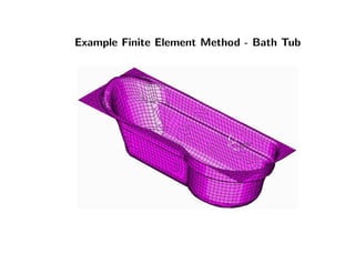
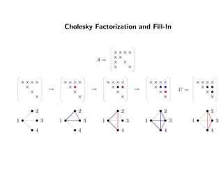
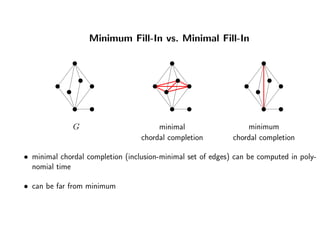
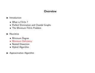
This document discusses the minimum fill-in problem for sparse matrices. It begins with an introduction to fill-in that occurs during Gaussian elimination due to the introduction of new non-zero elements. It describes how the minimum fill-in problem is NP-hard and discusses various heuristics to minimize fill-in, including minimum degree ordering and nested dissection. The minimum degree algorithm works by repeatedly eliminating the vertex with minimum degree but does not always produce optimal orderings. The document provides examples to illustrate minimum degree and discusses enhancements like mass elimination to improve its performance.

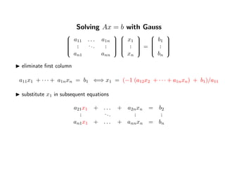

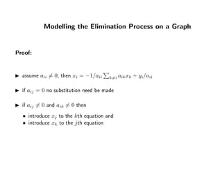
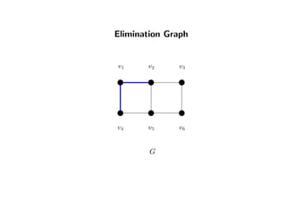
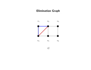
![Modelling the Elimination Process on a Graph
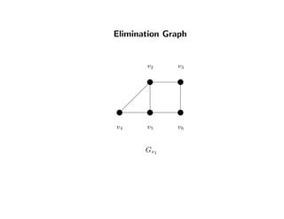
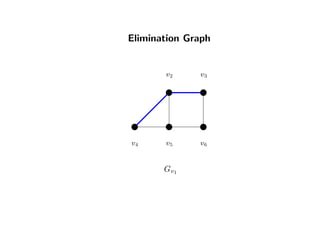
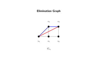
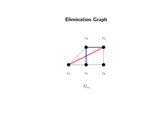
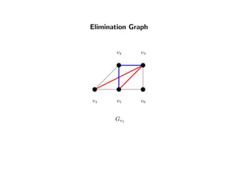
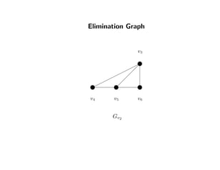
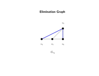
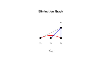
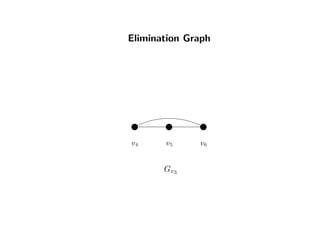
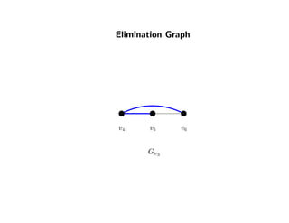
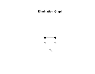
Let the graph G = (V, E) correspond to A and let the vertex vi correspond to xi.
Theorem: Elimination Graph [Parter 1961] Eliminating xi from the subsequent
equations, the new graph Gvi
of the remaining system is formed by:
1. eliminating the vertex vi that corresponds to xi from Gvi−1
2. pair-wise connecting the vertices of N(vi).
v1
v2 v2
v3 v3 v3
v4v4 v4v4
G Gv1
Gv2
Gv3
→→ →](https://image.slidesharecdn.com/c83dad54-13e3-4aa6-9ad0-417e4d6b42a0-151029082239-lva1-app6892/85/MinFill_Presentation-9-320.jpg)
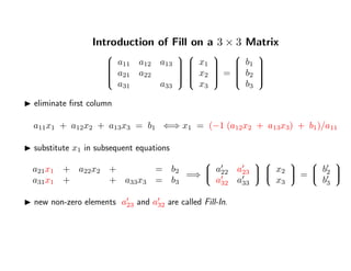
![EliminationGraph[Parter1961]
×
×
×
×
×
×
×
×
×
×
××
×
×
×
×
i
ii
i
ii
j
j
j
j
jj
k
k
k
k
kk
............
...
...
...
...
=⇒](https://image.slidesharecdn.com/c83dad54-13e3-4aa6-9ad0-417e4d6b42a0-151029082239-lva1-app6892/85/MinFill_Presentation-11-320.jpg)


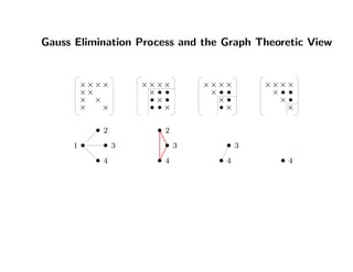
![Perfect Elimination
Definition: [Rose 1972] A is a perfect elimination matrix if there exists a permutation matrix
P such that ˜A = PAPT
= LLT
and aij = 0 ⇒ lij = 0, i < j.
Definition: For a graph G = (V, E) with |V | = n an ordering of V is a bijection
σ : {1, 2, . . . , n} → V .
1 1
22
3 3
4 4
v1v1 v1v1
v2v2 v2v2
v3v3 v3v3
v4 v4v4 v4
×
×
×
× ×
×
×
××
×
×
×
×
×
×
×
×
×
×
×
×
×
××
×
×
×
××
×
×
×××
•
••
→
LT
= LT
=](https://image.slidesharecdn.com/c83dad54-13e3-4aa6-9ad0-417e4d6b42a0-151029082239-lva1-app6892/85/MinFill_Presentation-15-320.jpg)
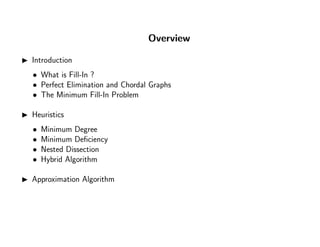
![Chordal Graph (Hanjal und Suranyi [1958])
Definition: A Graph G = (V, E) is chordal if every cycle of length ≥ 4 has a chord.
A chord is an edge connecting two nonconsecutive vertices of the cycle.
G1
chordal
G2
not chordal
G3
not chordal
The class of chordal graphs is the class of perfect elimination graphs.](https://image.slidesharecdn.com/c83dad54-13e3-4aa6-9ad0-417e4d6b42a0-151029082239-lva1-app6892/85/MinFill_Presentation-16-320.jpg)
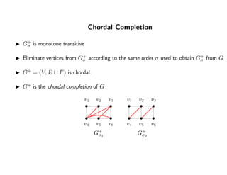
![Definition: The ordered graph Gσ is monotone transitive when
∀v ∈ V (v, u1) ∈ E and (v, u2) ∈ E =⇒ (u1, u2) ∈ E,
with σ−1
(v) < σ−1
(u1) and σ−1
(v) < σ−1
(u2)
Theorem: (Rose [1972]) For G = (V, E) the following statements are equivalent:
A is a perfect elimination matrix.
∃ an ordering σ of V such that Gσ is monotone transitive
σ is a perfect elimination order
G is chordal](https://image.slidesharecdn.com/c83dad54-13e3-4aa6-9ad0-417e4d6b42a0-151029082239-lva1-app6892/85/MinFill_Presentation-17-320.jpg)


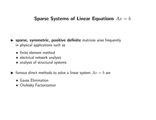
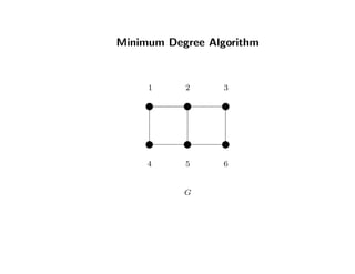
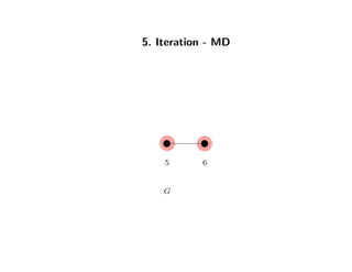
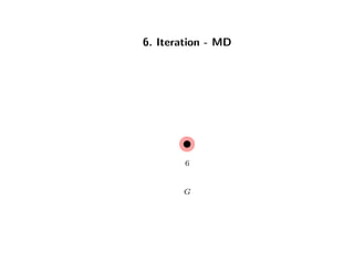
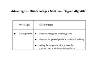
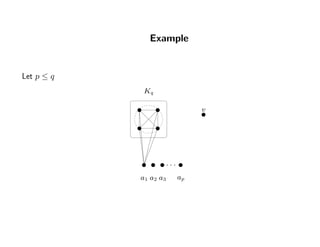
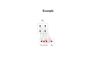
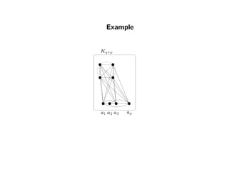
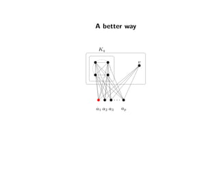
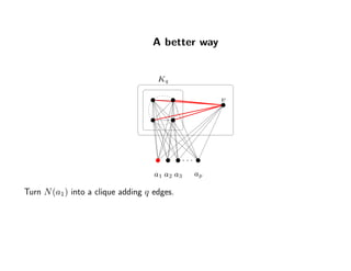
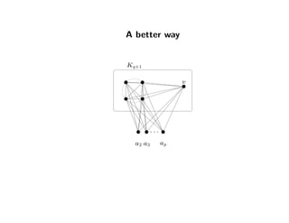
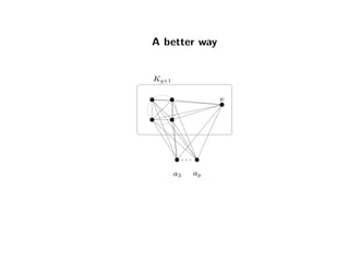
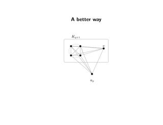
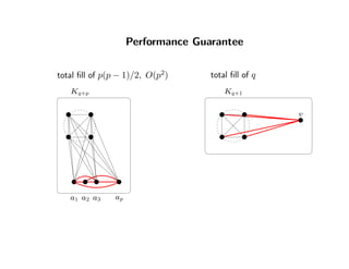
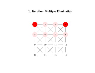
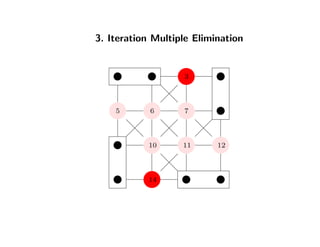
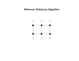
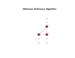
![Minimum Degree Algorithm
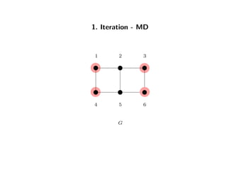
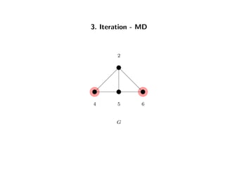
repeatedly finds a vertex of minimum degree and eliminates it
Enhancements
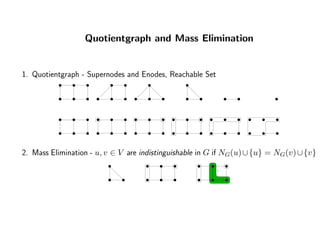
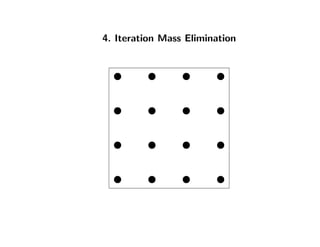
• Mass Elimination using Supernodes [George, Liu 1980]
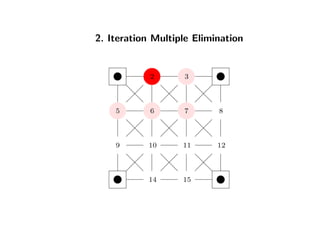
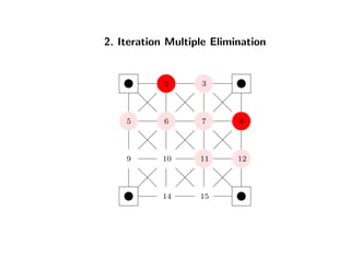
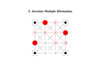
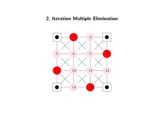
• Multiple Elimination [Liu 1985]
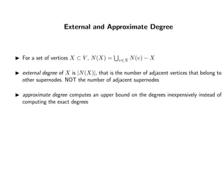
• External Degree [Liu 1985]
• Approximate Degree [Amestoy, Davis, Duff 1996]
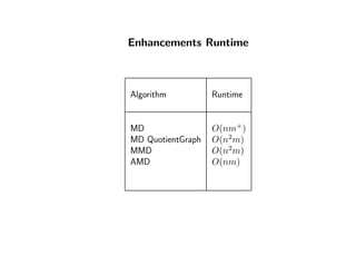
fast algorithm, runs in O(nm+
), where m+
= |E ∪ F|](https://image.slidesharecdn.com/c83dad54-13e3-4aa6-9ad0-417e4d6b42a0-151029082239-lva1-app6892/85/MinFill_Presentation-44-320.jpg)


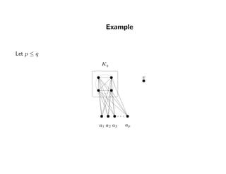


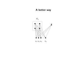
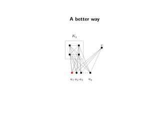


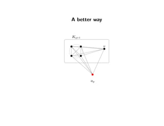
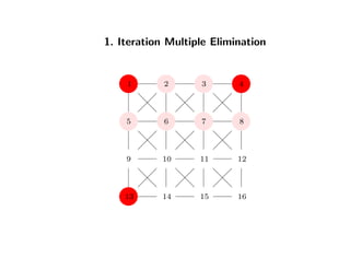
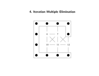
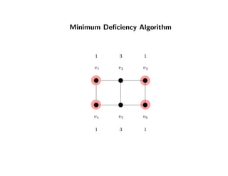
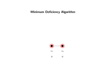
![Minimum Degree Algorithm
repeatedly finds a vertex of minimum degree and eliminates it
Enhancements
• Mass Elimination using Supernodes [George, Liu 1980]
• Multiple Elimination [Liu 1985]
• External Degree [Liu 1985]
• Approximate Degree [Amestoy, Davis, Duff 1996]
fast algorithm](https://image.slidesharecdn.com/c83dad54-13e3-4aa6-9ad0-417e4d6b42a0-151029082239-lva1-app6892/85/MinFill_Presentation-74-320.jpg)
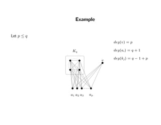
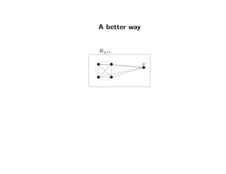
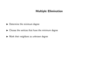
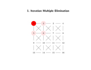
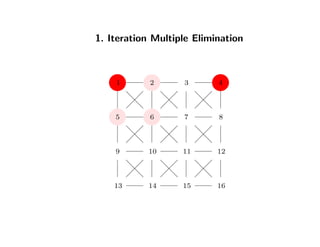
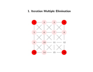
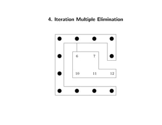
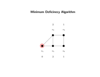
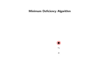
![Minimum Degree Algorithm
repeatedly finds a vertex of minimum degree and eliminates it
Enhancements
• Mass Elimination using Supernodes [George, Liu 1980]
• Multiple Elimination [Liu 1985]
• External Degree [Liu 1985]
• Approximate Degree [Amestoy, Davis, Duff 1996]
fast algorithm](https://image.slidesharecdn.com/c83dad54-13e3-4aa6-9ad0-417e4d6b42a0-151029082239-lva1-app6892/85/MinFill_Presentation-76-320.jpg)


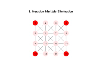


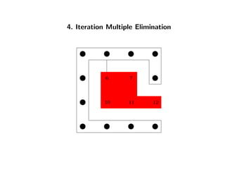
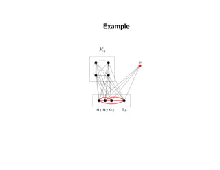
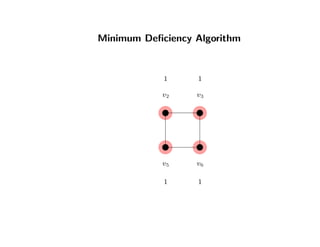
![Minimum Degree Algorithm
repeatedly finds a vertex of minimum degree and eliminates it
Enhancements
• Mass Elimination using Supernodes [George, Liu 1980]
• Multiple Elimination [Liu 1985]
• External Degree [Liu 1985]
• Approximate Degree [Amestoy, Davis, Duff 1996]
fast algorithm](https://image.slidesharecdn.com/c83dad54-13e3-4aa6-9ad0-417e4d6b42a0-151029082239-lva1-app6892/85/MinFill_Presentation-98-320.jpg)

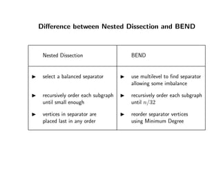
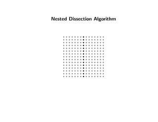
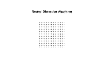
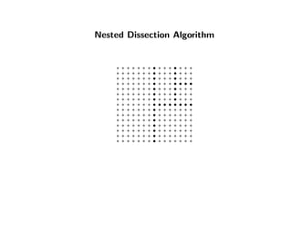
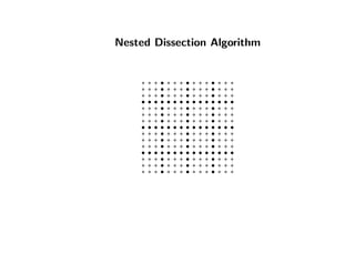
![Nested Dissection [George 1973]
Nested Dissection examines the graph as a whole before ordering
• orders the vertices of the graph backwards
• begins by deciding which vertices should be eliminated last
works by selecting a balanced separator
• a set of vertices, that when removed from the graph, partitions it into connected
components
vertices in the separator are placed last in the elimination order
recursively orders each of the connected components](https://image.slidesharecdn.com/c83dad54-13e3-4aa6-9ad0-417e4d6b42a0-151029082239-lva1-app6892/85/MinFill_Presentation-112-320.jpg)

![Performance Bound
At most O(n log n) fill for graphs with small separators (O(
√
n))[Lipton, Rose, Tarja 1979]
• planar graphs
• graphs with bounded genus
• graphs with bounded degree
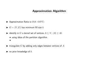
Approximation algorithm [Agraval, Klein, Ravi 1990] with performance bound O(
√
d log4
n)
• for bounded degree graphs
Theoretical result [Gilbert 1989]: for any graph there exisits a ND algorithm whose fill is
within O(d log n) of minimum, where d is the maximum degree.](https://image.slidesharecdn.com/c83dad54-13e3-4aa6-9ad0-417e4d6b42a0-151029082239-lva1-app6892/85/MinFill_Presentation-118-320.jpg)
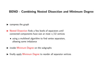
![Hybrid Algorithms
take advantage of of the best characteristics of
Minimum Degree and Nested Dissection
using a few levels of separators to control the fill
introduced by minimum degree orders
Hendrickson and Rothberg[1996] is the current champion
of ordering algorithms - BEND (Bruce and Ed’s Nested Dissection)
algorithm has neither known worst case fill nor work analysis](https://image.slidesharecdn.com/c83dad54-13e3-4aa6-9ad0-417e4d6b42a0-151029082239-lva1-app6892/85/MinFill_Presentation-122-320.jpg)