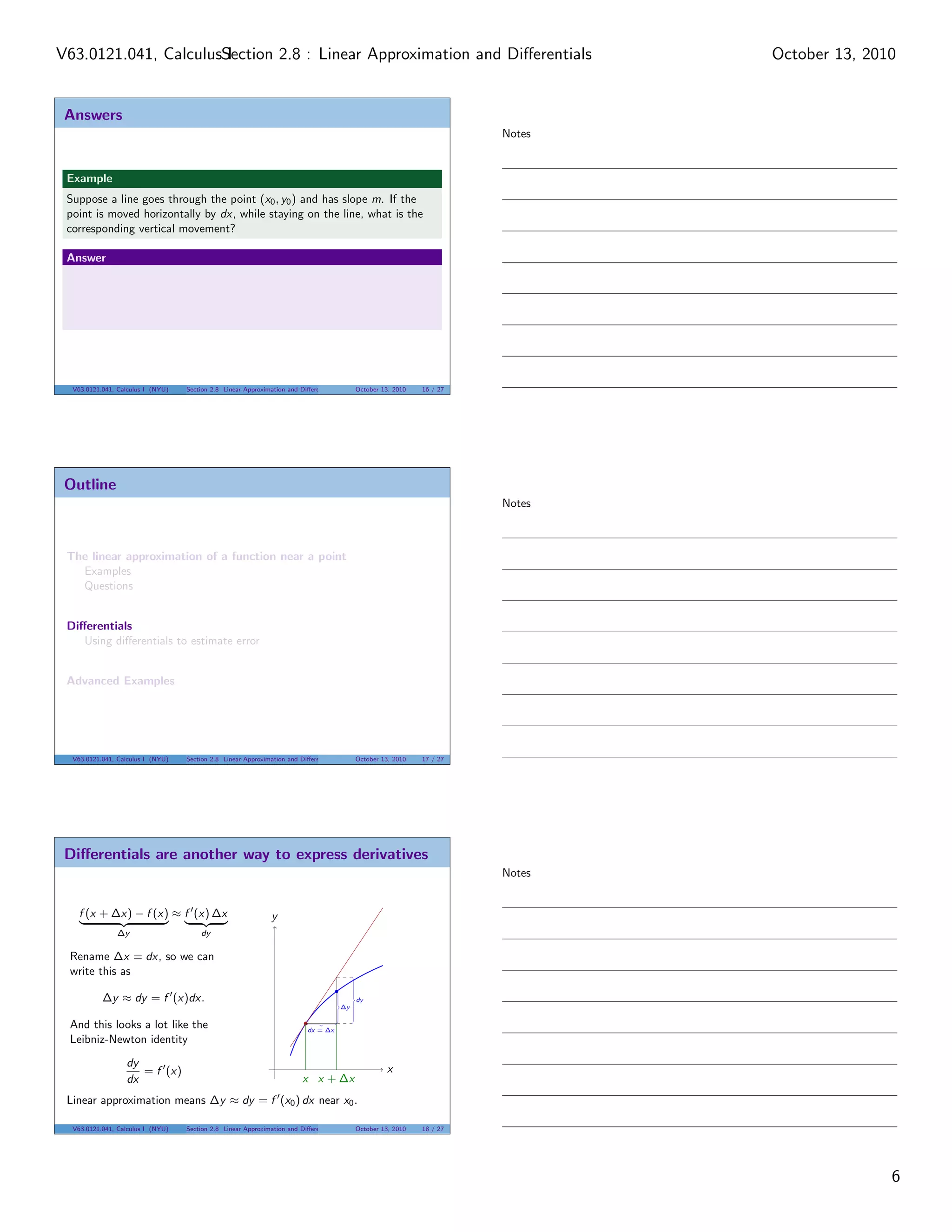
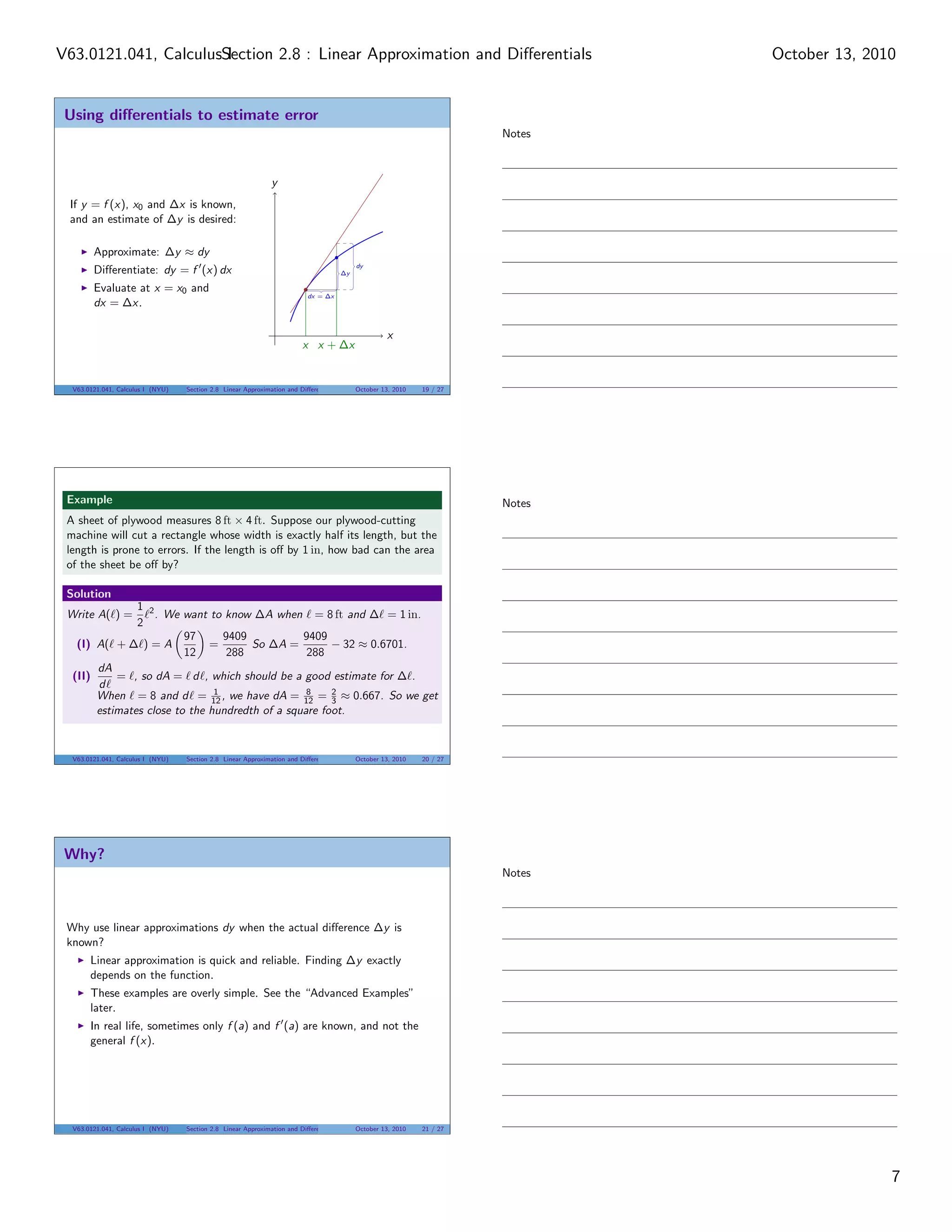
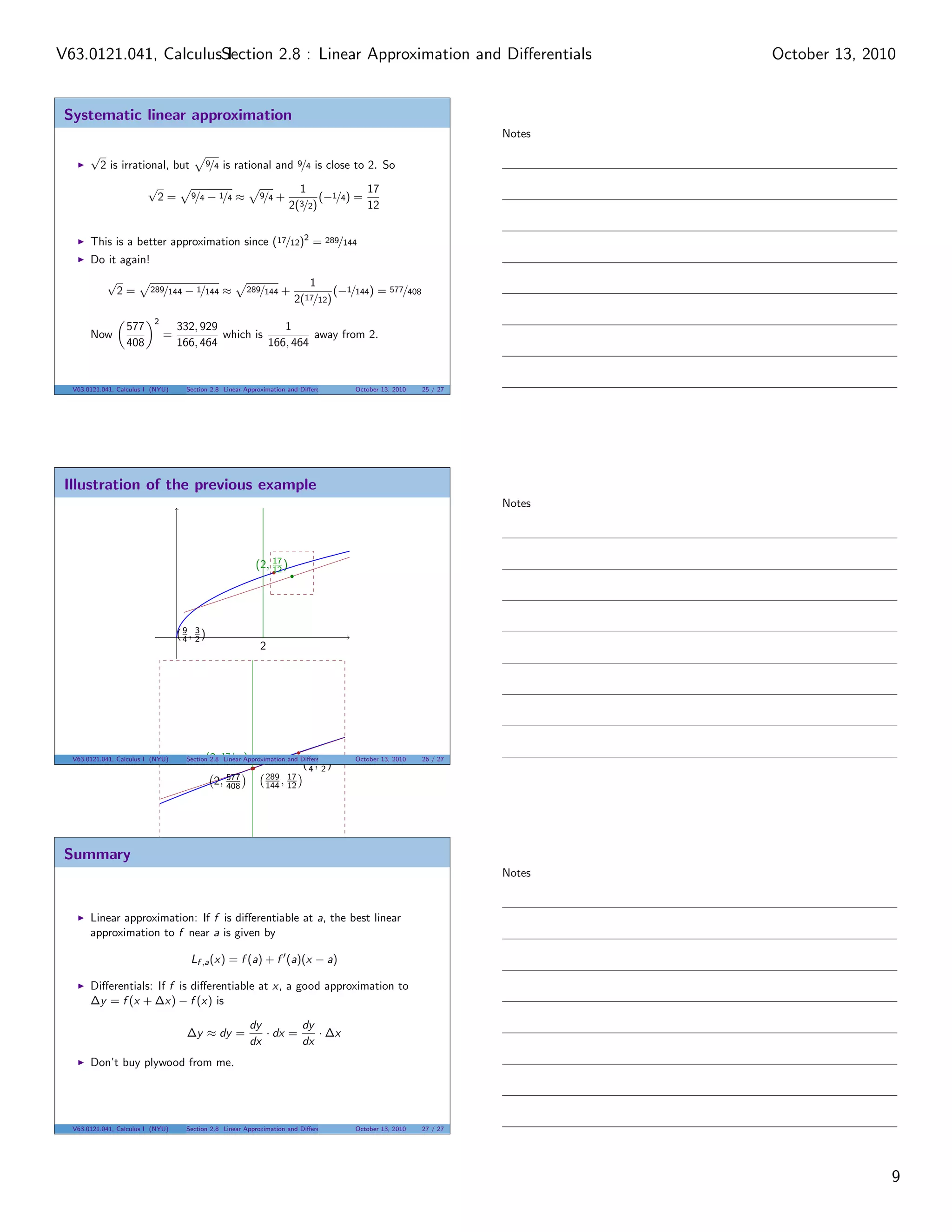
SlideShare a Scribd company logo
1 of 9
Download to read offline
V63.0121.041, CalculusSection 2.8 : Linear Approximation and Differentials
                       I                                                                                                   October 13, 2010


                                                                                                                   Notes
                            Section 2.8
               Linear Approximation and Differentials

                                    V63.0121.041, Calculus I

                                           New York University


                                          October 13, 2010


 Announcements

       Quiz 2 in recitation this week on §§1.5, 1.6, 2.1, 2.2
       Midterm on §§1.1–2.5


 Announcements
                                                                                                                   Notes


          Quiz 2 in recitation this
          week on §§1.5, 1.6, 2.1, 2.2
          Midterm on §§1.1–2.5


  V63.0121.041, Calculus I (NYU)   Section 2.8 Linear Approximation and Differentials   October 13, 2010   2 / 27


 Objectives
                                                                                                                   Notes
          Use tangent lines to make
          linear approximations to a
          function.
                 Given a function and a
                 point in the domain,
                 compute the linearization
                 of the function at that
                 point.
                 Use linearization to
                 approximate values of
                 functions
          Given a function, compute
          the differential of that
          function
          Use the differential notation
          to estimate error in linear
          approximations.
  V63.0121.041, Calculus I (NYU)   Section 2.8 Linear Approximation and Differentials   October 13, 2010   3 / 27


                                                                                                                                          1
V63.0121.041, CalculusSection 2.8 : Linear Approximation and Differentials
                       I                                                                                                    October 13, 2010


 Outline
                                                                                                                    Notes


 The linear approximation of a function near a point
   Examples
   Questions


 Differentials
    Using differentials to estimate error


 Advanced Examples


  V63.0121.041, Calculus I (NYU)   Section 2.8 Linear Approximation and Differentials    October 13, 2010   4 / 27


 The Big Idea
                                                                                                                    Notes
 Question
 Let f be differentiable at a. What linear function best approximates f near
 a?

 Answer
 The tangent line, of course!

 Question
 What is the equation for the line tangent to y = f (x) at (a, f (a))?

 Answer

                                   L(x) = f (a) + f (a)(x − a)


  V63.0121.041, Calculus I (NYU)   Section 2.8 Linear Approximation and Differentials    October 13, 2010   5 / 27


 The tangent line is a linear approximation
                                                                                                                    Notes


                                                               y


      L(x) = f (a) + f (a)(x − a)

 is a decent approximation to f                        L(x)
 near a.                                               f (x)
 How decent? The closer x is to
 a, the better the approxmation                        f (a)                 x −a
 L(x) is to f (x)

                                                                                                x
                                                                         a          x


  V63.0121.041, Calculus I (NYU)   Section 2.8 Linear Approximation and Differentials    October 13, 2010   6 / 27


                                                                                                                                           2
V63.0121.041, CalculusSection 2.8 : Linear Approximation and Differentials
                       I                                                                                                           October 13, 2010


 Example
                                                                                                                           Notes
 Example
 Estimate sin(61◦ ) = sin(61π/180) by using a linear approximation
 (i) about a = 0      (ii) about a = 60◦ = π/3.

 Solution (i)                                               Solution (ii)
                                                                                                √
      If f (x) = sin x, then f (0) = 0                             We have f π = 23 and
                                                                               3
      and f (0) = 1.                                               f π = 1.
                                                                      3     2 √
      So the linear approximation near                                          3 1     π
                                                                   So L(x) =     +   x−
      0 is L(x) = 0 + 1 · x = x.                                               2   2    3
                                                                   Thus
      Thus
                                                                                   61π
                61π          61π                                           sin               ≈ 0.87475
         sin             ≈       ≈ 1.06465                                         180
                180          180

 Calculator check: sin(61◦ ) ≈ 0.87462.


  V63.0121.041, Calculus I (NYU)   Section 2.8 Linear Approximation and Differentials       October 13, 2010       7 / 27


 Illustration
                                                                                                                           Notes
        y
                                                                   y = L1 (x) = x


                                                                                         √
                                                                                            3       1         π
                                                       y = L2 (x) =                        2    +   2   x−    3
                           big difference!                y = sin x
                                          very little difference!


                                                                                       x
            0                           π/3      61◦

  V63.0121.041, Calculus I (NYU)   Section 2.8 Linear Approximation and Differentials       October 13, 2010       8 / 27


 Another Example
                                                                                                                           Notes
 Example
                √
 Estimate           10 using the fact that 10 = 9 + 1.

 Solution


  V63.0121.041, Calculus I (NYU)   Section 2.8 Linear Approximation and Differentials       October 13, 2010       9 / 27


                                                                                                                                                  3
V63.0121.041, CalculusSection 2.8 : Linear Approximation and Differentials
                       I                                                                                                    October 13, 2010


 Dividing without dividing?
                                                                                                                    Notes
 Example
 Suppose I have an irrational fear of division and need to estimate
 577 ÷ 408. I write
                         577            1             1  1
                             = 1 + 169     = 1 + 169 × ×    .
                         408           408            4 102
                                    1
 But still I have to find               .
                                   102

 Solution


  V63.0121.041, Calculus I (NYU)   Section 2.8 Linear Approximation and Differentials   October 13, 2010   10 / 27


 Questions
                                                                                                                    Notes

 Example
 Suppose we are traveling in a car and at noon our speed is 50 mi/hr. How
 far will we have traveled by 2:00pm? by 3:00pm? By midnight?

 Example
 Suppose our factory makes MP3 players and the marginal cost is currently
 $50/lot. How much will it cost to make 2 more lots? 3 more lots? 12
 more lots?

 Example
 Suppose a line goes through the point (x0 , y0 ) and has slope m. If the
 point is moved horizontally by dx, while staying on the line, what is the
 corresponding vertical movement?


  V63.0121.041, Calculus I (NYU)   Section 2.8 Linear Approximation and Differentials   October 13, 2010   11 / 27


 Answers
                                                                                                                    Notes


 Example
 Suppose we are traveling in a car and at noon our speed is 50 mi/hr. How
 far will we have traveled by 2:00pm? by 3:00pm? By midnight?

 Answer


  V63.0121.041, Calculus I (NYU)   Section 2.8 Linear Approximation and Differentials   October 13, 2010   12 / 27


                                                                                                                                           4
V63.0121.041, CalculusSection 2.8 : Linear Approximation and Differentials
                       I                                                                                                    October 13, 2010


 Questions
                                                                                                                    Notes

 Example
 Suppose we are traveling in a car and at noon our speed is 50 mi/hr. How
 far will we have traveled by 2:00pm? by 3:00pm? By midnight?

 Example
 Suppose our factory makes MP3 players and the marginal cost is currently
 $50/lot. How much will it cost to make 2 more lots? 3 more lots? 12
 more lots?

 Example
 Suppose a line goes through the point (x0 , y0 ) and has slope m. If the
 point is moved horizontally by dx, while staying on the line, what is the
 corresponding vertical movement?


  V63.0121.041, Calculus I (NYU)   Section 2.8 Linear Approximation and Differentials   October 13, 2010   13 / 27


 Answers
                                                                                                                    Notes


 Example
 Suppose our factory makes MP3 players and the marginal cost is currently
 $50/lot. How much will it cost to make 2 more lots? 3 more lots? 12
 more lots?

 Answer


  V63.0121.041, Calculus I (NYU)   Section 2.8 Linear Approximation and Differentials   October 13, 2010   14 / 27


 Questions
                                                                                                                    Notes

 Example
 Suppose we are traveling in a car and at noon our speed is 50 mi/hr. How
 far will we have traveled by 2:00pm? by 3:00pm? By midnight?

 Example
 Suppose our factory makes MP3 players and the marginal cost is currently
 $50/lot. How much will it cost to make 2 more lots? 3 more lots? 12
 more lots?

 Example
 Suppose a line goes through the point (x0 , y0 ) and has slope m. If the
 point is moved horizontally by dx, while staying on the line, what is the
 corresponding vertical movement?


  V63.0121.041, Calculus I (NYU)   Section 2.8 Linear Approximation and Differentials   October 13, 2010   15 / 27


                                                                                                                                           5
V63.0121.041, CalculusSection 2.8 : Linear Approximation and Differentials
                       I                                                                                                         October 13, 2010


 Answers
                                                                                                                         Notes


 Example
 Suppose a line goes through the point (x0 , y0 ) and has slope m. If the
 point is moved horizontally by dx, while staying on the line, what is the
 corresponding vertical movement?

 Answer


  V63.0121.041, Calculus I (NYU)   Section 2.8 Linear Approximation and Differentials        October 13, 2010   16 / 27


 Outline
                                                                                                                         Notes


 The linear approximation of a function near a point
   Examples
   Questions


 Differentials
    Using differentials to estimate error


 Advanced Examples


  V63.0121.041, Calculus I (NYU)   Section 2.8 Linear Approximation and Differentials        October 13, 2010   17 / 27


 Differentials are another way to express derivatives
                                                                                                                         Notes


    f (x + ∆x) − f (x) ≈ f (x) ∆x                              y
                ∆y                     dy

 Rename ∆x = dx, so we can
 write this as

           ∆y ≈ dy = f (x)dx.                                                               dy
                                                                                       ∆y

 And this looks a lot like the                                             dx = ∆x
 Leibniz-Newton identity
                  dy
                     = f (x)                                                                          x
                  dx                                                     x x + ∆x
 Linear approximation means ∆y ≈ dy = f (x0 ) dx near x0 .

  V63.0121.041, Calculus I (NYU)   Section 2.8 Linear Approximation and Differentials        October 13, 2010   18 / 27


                                                                                                                                                6
V63.0121.041, CalculusSection 2.8 : Linear Approximation and Differentials
                       I                                                                                                         October 13, 2010


 Using differentials to estimate error
                                                                                                                         Notes


                                                               y
 If y = f (x), x0 and ∆x is known,
 and an estimate of ∆y is desired:

        Approximate: ∆y ≈ dy
                                                                                            dy
        Differentiate: dy = f (x) dx                                                    ∆y

        Evaluate at x = x0 and
                                                                           dx = ∆x
        dx = ∆x.

                                                                                                      x
                                                                         x x + ∆x


  V63.0121.041, Calculus I (NYU)   Section 2.8 Linear Approximation and Differentials        October 13, 2010   19 / 27


 Example                                                                                                                 Notes
 A sheet of plywood measures 8 ft × 4 ft. Suppose our plywood-cutting
 machine will cut a rectangle whose width is exactly half its length, but the
 length is prone to errors. If the length is off by 1 in, how bad can the area
 of the sheet be off by?

 Solution
               1 2
 Write A( ) =      . We want to know ∆A when = 8 ft and ∆ = 1 in.
               2
                         97      9409           9409
   (I) A( + ∆ ) = A           =       So ∆A =         − 32 ≈ 0.6701.
                         12      288             288
       dA
  (II)     = , so dA = d , which should be a good estimate for ∆ .
       d
       When = 8 and d = 12 , we have dA = 12 = 2 ≈ 0.667. So we get
                               1                 8
                                                      3
       estimates close to the hundredth of a square foot.


  V63.0121.041, Calculus I (NYU)   Section 2.8 Linear Approximation and Differentials        October 13, 2010   20 / 27


 Why?
                                                                                                                         Notes


 Why use linear approximations dy when the actual difference ∆y is
 known?
       Linear approximation is quick and reliable. Finding ∆y exactly
       depends on the function.
       These examples are overly simple. See the “Advanced Examples”
       later.
       In real life, sometimes only f (a) and f (a) are known, and not the
       general f (x).


  V63.0121.041, Calculus I (NYU)   Section 2.8 Linear Approximation and Differentials        October 13, 2010   21 / 27


                                                                                                                                                7
V63.0121.041, CalculusSection 2.8 : Linear Approximation and Differentials
                       I                                                                                                      October 13, 2010


 Outline
                                                                                                                      Notes


 The linear approximation of a function near a point
   Examples
   Questions


 Differentials
    Using differentials to estimate error


 Advanced Examples


  V63.0121.041, Calculus I (NYU)     Section 2.8 Linear Approximation and Differentials   October 13, 2010   22 / 27


 Gravitation
 Pencils down!                                                                                                        Notes

 Example

       Drop a 1 kg ball off the roof of the Silver Center (50m high). We
       usually say that a falling object feels a force F = −mg from gravity.
       In fact, the force felt is
                                                                 GMm
                                                 F (r ) = −          ,
                                                                  r2
       where M is the mass of the earth and r is the distance from the
       center of the earth to the object. G is a constant.
                                               GMm
       At r = re the force really is F (re ) =   2
                                                    = −mg .
                                                re
       What is the maximum error in replacing the actual force felt at the
       top of the building F (re + ∆r ) by the force felt at ground level F (re )?
       The relative error? The percentage error?
  V63.0121.041, Calculus I (NYU)     Section 2.8 Linear Approximation and Differentials   October 13, 2010   23 / 27


 Gravitation Solution
                                                                                                                      Notes
 Solution
 We wonder if ∆F = F (re + ∆r ) − F (re ) is small.
       Using a linear approximation,

                                                      dF                   GMm
                                   ∆F ≈ dF =                     dr = 2      3
                                                                               dr
                                                      dr    re              re
                                                        GMm           dr       ∆r
                                                 =        2
                                                                         = 2mg
                                                         re           re       re

                           ∆F        ∆r
       The relative error is   ≈ −2
                            F        re
       re = 6378.1 km. If ∆r = 50 m,
              ∆F      ∆r         50
                 ≈ −2    = −2         = −1.56 × 10−5 = −0.00156%
              F       re      6378100

  V63.0121.041, Calculus I (NYU)     Section 2.8 Linear Approximation and Differentials   October 13, 2010   24 / 27


                                                                                                                                             8
V63.0121.041, CalculusSection 2.8 : Linear Approximation and Differentials
                       I                                                                                                      October 13, 2010


 Systematic linear approximation
                                                                                                                      Notes
       √
           2 is irrational, but             9/4   is rational and 9/4 is close to 2. So
                         √                                               1             17
                             2=       9/4   − 1/4 ≈          9/4   +          (−1/4) =
                                                                       2(3/2)          12


       This is a better approximation since (17/12)2 = 289/144
       Do it again!
            √                                                              1
                2=        289/144   − 1/144 ≈            289/144    +            (−1/144) = 577/408
                                                                        2(17/12)
                           2
                  577              332, 929             1
       Now                     =            which is          away from 2.
                  408              166, 464          166, 464


  V63.0121.041, Calculus I (NYU)     Section 2.8 Linear Approximation and Differentials   October 13, 2010   25 / 27


 Illustration of the previous example
                                                                                                                      Notes


                                                           (2, 17 )
                                                               12


                                   (9, 2)
                                    4
                                       3
                                                             2


  V63.0121.041, Calculus I (NYU)     Section 2.8 17 12Approximation and Differentials
                                            (2, / )
                                                 Linear                   9 3            October 13, 2010   26 / 27
                                                                           (4, 2)
                                                   577         289 17
                                              2,   408         144 , 12


 Summary
                                                                                                                      Notes


       Linear approximation: If f is differentiable at a, the best linear
       approximation to f near a is given by

                                      Lf ,a (x) = f (a) + f (a)(x − a)

       Differentials: If f is differentiable at x, a good approximation to
       ∆y = f (x + ∆x) − f (x) is

                                                         dy        dy
                                     ∆y ≈ dy =              · dx =    · ∆x
                                                         2
                                                         dx        dx
       Don’t buy plywood from me.


  V63.0121.041, Calculus I (NYU)     Section 2.8 Linear Approximation and Differentials   October 13, 2010   27 / 27


                                                                                                                                             9

More Related Content

What's hot

Lesson 23: The Definite Integral (handout)
Lesson 23: The Definite Integral (handout)Lesson 23: The Definite Integral (handout)
Lesson 23: The Definite Integral (handout)Matthew Leingang
 
Lesson 15: Exponential Growth and Decay
Lesson 15: Exponential Growth and DecayLesson 15: Exponential Growth and Decay
Lesson 15: Exponential Growth and DecayMatthew Leingang
 
Lesson 23: Antiderivatives (Section 021 slides)
Lesson 23: Antiderivatives (Section 021 slides)Lesson 23: Antiderivatives (Section 021 slides)
Lesson 23: Antiderivatives (Section 021 slides)Matthew Leingang
 
Lesson 20: Derivatives and the Shapes of Curves (handout)
Lesson 20: Derivatives and the Shapes of Curves (handout)Lesson 20: Derivatives and the Shapes of Curves (handout)
Lesson 20: Derivatives and the Shapes of Curves (handout)Matthew Leingang
 
Lesson 2: A Catalog of Essential Functions
Lesson 2: A Catalog of Essential FunctionsLesson 2: A Catalog of Essential Functions
Lesson 2: A Catalog of Essential FunctionsMatthew Leingang
 
Lesson 23: Antiderivatives (Section 041 slides)
Lesson 23: Antiderivatives (Section 041 slides)Lesson 23: Antiderivatives (Section 041 slides)
Lesson 23: Antiderivatives (Section 041 slides)Matthew Leingang
 
Lesson 6: Limits Involving Infinity (Section 41 handout)
Lesson 6: Limits Involving Infinity (Section 41 handout)Lesson 6: Limits Involving Infinity (Section 41 handout)
Lesson 6: Limits Involving Infinity (Section 41 handout)Matthew Leingang
 
Lesson 22: Optimization (Section 021 slides)
Lesson 22: Optimization (Section 021 slides)Lesson 22: Optimization (Section 021 slides)
Lesson 22: Optimization (Section 021 slides)Matthew Leingang
 
Lesson16 -inverse_trigonometric_functions_021_handout
Lesson16  -inverse_trigonometric_functions_021_handoutLesson16  -inverse_trigonometric_functions_021_handout
Lesson16 -inverse_trigonometric_functions_021_handoutMatthew Leingang
 
Expo Algebra Lineal
Expo Algebra LinealExpo Algebra Lineal
Expo Algebra LinealNoi
 
Lesson 27: Integration by Substitution (Section 041 handout)
Lesson 27: Integration by Substitution (Section 041 handout)Lesson 27: Integration by Substitution (Section 041 handout)
Lesson 27: Integration by Substitution (Section 041 handout)Matthew Leingang
 
Lesson 5: Continuity (Section 21 handout)
Lesson 5: Continuity (Section 21 handout)Lesson 5: Continuity (Section 21 handout)
Lesson 5: Continuity (Section 21 handout)Matthew Leingang
 
Kccsi 2012 a real-time robust object tracking-v2
Kccsi 2012   a real-time robust object tracking-v2Kccsi 2012   a real-time robust object tracking-v2
Kccsi 2012 a real-time robust object tracking-v2Prarinya Siritanawan
 
Lesson 27: Integration by Substitution (Section 021 handout)
Lesson 27: Integration by Substitution (Section 021 handout)Lesson 27: Integration by Substitution (Section 021 handout)
Lesson 27: Integration by Substitution (Section 021 handout)Matthew Leingang
 
Lesson 11: Implicit Differentiation (Section 21 handout)
Lesson 11: Implicit Differentiation (Section 21 handout)Lesson 11: Implicit Differentiation (Section 21 handout)
Lesson 11: Implicit Differentiation (Section 21 handout)Matthew Leingang
 
Lesson 16: Inverse Trigonometric Functions (Section 041 handout)
Lesson 16: Inverse Trigonometric Functions (Section 041 handout)Lesson 16: Inverse Trigonometric Functions (Section 041 handout)
Lesson 16: Inverse Trigonometric Functions (Section 041 handout)Matthew Leingang
 
Cs221 linear algebra
Cs221 linear algebraCs221 linear algebra
Cs221 linear algebradarwinrlo
 

What's hot (19)

Lesson 23: The Definite Integral (handout)
Lesson 23: The Definite Integral (handout)Lesson 23: The Definite Integral (handout)
Lesson 23: The Definite Integral (handout)
 
Lesson 15: Exponential Growth and Decay
Lesson 15: Exponential Growth and DecayLesson 15: Exponential Growth and Decay
Lesson 15: Exponential Growth and Decay
 
Lesson 23: Antiderivatives (Section 021 slides)
Lesson 23: Antiderivatives (Section 021 slides)Lesson 23: Antiderivatives (Section 021 slides)
Lesson 23: Antiderivatives (Section 021 slides)
 
Lesson 20: Derivatives and the Shapes of Curves (handout)
Lesson 20: Derivatives and the Shapes of Curves (handout)Lesson 20: Derivatives and the Shapes of Curves (handout)
Lesson 20: Derivatives and the Shapes of Curves (handout)
 
Lesson 2: A Catalog of Essential Functions
Lesson 2: A Catalog of Essential FunctionsLesson 2: A Catalog of Essential Functions
Lesson 2: A Catalog of Essential Functions
 
Lesson 23: Antiderivatives (Section 041 slides)
Lesson 23: Antiderivatives (Section 041 slides)Lesson 23: Antiderivatives (Section 041 slides)
Lesson 23: Antiderivatives (Section 041 slides)
 
Lesson 6: Limits Involving Infinity (Section 41 handout)
Lesson 6: Limits Involving Infinity (Section 41 handout)Lesson 6: Limits Involving Infinity (Section 41 handout)
Lesson 6: Limits Involving Infinity (Section 41 handout)
 
Lesson 22: Optimization (Section 021 slides)
Lesson 22: Optimization (Section 021 slides)Lesson 22: Optimization (Section 021 slides)
Lesson 22: Optimization (Section 021 slides)
 
Lesson16 -inverse_trigonometric_functions_021_handout
Lesson16  -inverse_trigonometric_functions_021_handoutLesson16  -inverse_trigonometric_functions_021_handout
Lesson16 -inverse_trigonometric_functions_021_handout
 
Expo Algebra Lineal
Expo Algebra LinealExpo Algebra Lineal
Expo Algebra Lineal
 
Lesson 27: Integration by Substitution (Section 041 handout)
Lesson 27: Integration by Substitution (Section 041 handout)Lesson 27: Integration by Substitution (Section 041 handout)
Lesson 27: Integration by Substitution (Section 041 handout)
 
Lesson 5: Continuity (Section 21 handout)
Lesson 5: Continuity (Section 21 handout)Lesson 5: Continuity (Section 21 handout)
Lesson 5: Continuity (Section 21 handout)
 
05 Random Variables
05 Random Variables05 Random Variables
05 Random Variables
 
Kccsi 2012 a real-time robust object tracking-v2
Kccsi 2012   a real-time robust object tracking-v2Kccsi 2012   a real-time robust object tracking-v2
Kccsi 2012 a real-time robust object tracking-v2
 
Linear Algebra
Linear AlgebraLinear Algebra
Linear Algebra
 
Lesson 27: Integration by Substitution (Section 021 handout)
Lesson 27: Integration by Substitution (Section 021 handout)Lesson 27: Integration by Substitution (Section 021 handout)
Lesson 27: Integration by Substitution (Section 021 handout)
 
Lesson 11: Implicit Differentiation (Section 21 handout)
Lesson 11: Implicit Differentiation (Section 21 handout)Lesson 11: Implicit Differentiation (Section 21 handout)
Lesson 11: Implicit Differentiation (Section 21 handout)
 
Lesson 16: Inverse Trigonometric Functions (Section 041 handout)
Lesson 16: Inverse Trigonometric Functions (Section 041 handout)Lesson 16: Inverse Trigonometric Functions (Section 041 handout)
Lesson 16: Inverse Trigonometric Functions (Section 041 handout)
 
Cs221 linear algebra
Cs221 linear algebraCs221 linear algebra
Cs221 linear algebra
 

Viewers also liked

Lesson 7: The Derivative (Section 41 slides)
Lesson 7: The Derivative (Section 41 slides)Lesson 7: The Derivative (Section 41 slides)
Lesson 7: The Derivative (Section 41 slides)Matthew Leingang
 
Lesson24 Implicit Differentiation Slides
Lesson24    Implicit  Differentiation SlidesLesson24    Implicit  Differentiation Slides
Lesson24 Implicit Differentiation SlidesMatthew Leingang
 
Lesson 2: A Catalog of Essential Functions
Lesson 2: A Catalog of Essential FunctionsLesson 2: A Catalog of Essential Functions
Lesson 2: A Catalog of Essential FunctionsMatthew Leingang
 

Viewers also liked (7)

Lesson 7: The Derivative (Section 41 slides)
Lesson 7: The Derivative (Section 41 slides)Lesson 7: The Derivative (Section 41 slides)
Lesson 7: The Derivative (Section 41 slides)
 
Lesson24 Implicit Differentiation Slides
Lesson24    Implicit  Differentiation SlidesLesson24    Implicit  Differentiation Slides
Lesson24 Implicit Differentiation Slides
 
Lesson 1: Functions
Lesson 1: FunctionsLesson 1: Functions
Lesson 1: Functions
 
Math 20 Introduction
Math 20 IntroductionMath 20 Introduction
Math 20 Introduction
 
Lesson 2: A Catalog of Essential Functions
Lesson 2: A Catalog of Essential FunctionsLesson 2: A Catalog of Essential Functions
Lesson 2: A Catalog of Essential Functions
 
Öncel Akademi: Konferans
Öncel Akademi: KonferansÖncel Akademi: Konferans
Öncel Akademi: Konferans
 
Making Lesson Plans
Making Lesson PlansMaking Lesson Plans
Making Lesson Plans
 

Similar to Lesson 12: Linear Approximation (Section 41 handout)

Lesson 12: Linear Approximations and Differentials (handout)
Lesson 12: Linear Approximations and Differentials (handout)Lesson 12: Linear Approximations and Differentials (handout)
Lesson 12: Linear Approximations and Differentials (handout)Matthew Leingang
 
Lesson 10: The Chain Rule (Section 21 handout)
Lesson 10: The Chain Rule (Section 21 handout)Lesson 10: The Chain Rule (Section 21 handout)
Lesson 10: The Chain Rule (Section 21 handout)Matthew Leingang
 
Lesson 12: Linear Approximation and Differentials (Section 41 slides)
Lesson 12: Linear Approximation and Differentials (Section 41 slides)Lesson 12: Linear Approximation and Differentials (Section 41 slides)
Lesson 12: Linear Approximation and Differentials (Section 41 slides)Mel Anthony Pepito
 
Lesson 12: Linear Approximation and Differentials (Section 41 slides)
Lesson 12: Linear Approximation and Differentials (Section 41 slides)Lesson 12: Linear Approximation and Differentials (Section 41 slides)
Lesson 12: Linear Approximation and Differentials (Section 41 slides)Matthew Leingang
 
Lesson 10: The Chain Rule (Section 41 handout)
Lesson 10: The Chain Rule (Section 41 handout)Lesson 10: The Chain Rule (Section 41 handout)
Lesson 10: The Chain Rule (Section 41 handout)Matthew Leingang
 
Lesson 12: Linear Approximation
Lesson 12: Linear ApproximationLesson 12: Linear Approximation
Lesson 12: Linear ApproximationMatthew Leingang
 
Lesson 12: Linear Approximation
Lesson 12: Linear ApproximationLesson 12: Linear Approximation
Lesson 12: Linear ApproximationMel Anthony Pepito
 
Lesson 13: Exponential and Logarithmic Functions (Section 041 handout)
Lesson 13: Exponential and Logarithmic Functions (Section 041 handout)Lesson 13: Exponential and Logarithmic Functions (Section 041 handout)
Lesson 13: Exponential and Logarithmic Functions (Section 041 handout)Matthew Leingang
 
Lesson16 -inverse_trigonometric_functions_021_handout
Lesson16  -inverse_trigonometric_functions_021_handoutLesson16  -inverse_trigonometric_functions_021_handout
Lesson16 -inverse_trigonometric_functions_021_handoutMatthew Leingang
 
Lesson 2: A Catalog of Essential Functions
Lesson 2: A Catalog of Essential FunctionsLesson 2: A Catalog of Essential Functions
Lesson 2: A Catalog of Essential FunctionsMatthew Leingang
 
Lesson 2: A Catalog of Essential Functions
Lesson 2: A Catalog of Essential FunctionsLesson 2: A Catalog of Essential Functions
Lesson 2: A Catalog of Essential FunctionsMel Anthony Pepito
 
Lesson 10: The Chain Rule (handout)
Lesson 10: The Chain Rule (handout)Lesson 10: The Chain Rule (handout)
Lesson 10: The Chain Rule (handout)Matthew Leingang
 
Lesson 19: The Mean Value Theorem (Section 021 handout)
Lesson 19: The Mean Value Theorem (Section 021 handout)Lesson 19: The Mean Value Theorem (Section 021 handout)
Lesson 19: The Mean Value Theorem (Section 021 handout)Matthew Leingang
 
Lesson 14: Derivatives of Exponential and Logarithmic Functions (Section 021 ...
Lesson 14: Derivatives of Exponential and Logarithmic Functions (Section 021 ...Lesson 14: Derivatives of Exponential and Logarithmic Functions (Section 021 ...
Lesson 14: Derivatives of Exponential and Logarithmic Functions (Section 021 ...Mel Anthony Pepito
 
Lesson 2: A Catalog of Essential Functions
Lesson 2: A Catalog of Essential FunctionsLesson 2: A Catalog of Essential Functions
Lesson 2: A Catalog of Essential FunctionsMel Anthony Pepito
 
Lesson 19: The Mean Value Theorem (Section 041 handout)
Lesson 19: The Mean Value Theorem (Section 041 handout)Lesson 19: The Mean Value Theorem (Section 041 handout)
Lesson 19: The Mean Value Theorem (Section 041 handout)Matthew Leingang
 
Lesson 20: Derivatives and the Shape of Curves (Section 041 handout)
Lesson 20: Derivatives and the Shape of Curves (Section 041 handout)Lesson 20: Derivatives and the Shape of Curves (Section 041 handout)
Lesson 20: Derivatives and the Shape of Curves (Section 041 handout)Matthew Leingang
 
Lesson 20: Derivatives and the Shape of Curves (Section 041 slides)
Lesson 20: Derivatives and the Shape of Curves (Section 041 slides)Lesson 20: Derivatives and the Shape of Curves (Section 041 slides)
Lesson 20: Derivatives and the Shape of Curves (Section 041 slides)Mel Anthony Pepito
 
Lesson 7: The Derivative (Section 41 handout)
Lesson 7: The Derivative (Section 41 handout)Lesson 7: The Derivative (Section 41 handout)
Lesson 7: The Derivative (Section 41 handout)Matthew Leingang
 

Similar to Lesson 12: Linear Approximation (Section 41 handout) (20)

Lesson 12: Linear Approximations and Differentials (handout)
Lesson 12: Linear Approximations and Differentials (handout)Lesson 12: Linear Approximations and Differentials (handout)
Lesson 12: Linear Approximations and Differentials (handout)
 
Lesson 10: The Chain Rule (Section 21 handout)
Lesson 10: The Chain Rule (Section 21 handout)Lesson 10: The Chain Rule (Section 21 handout)
Lesson 10: The Chain Rule (Section 21 handout)
 
Lesson 12: Linear Approximation and Differentials (Section 41 slides)
Lesson 12: Linear Approximation and Differentials (Section 41 slides)Lesson 12: Linear Approximation and Differentials (Section 41 slides)
Lesson 12: Linear Approximation and Differentials (Section 41 slides)
 
Lesson 12: Linear Approximation and Differentials (Section 41 slides)
Lesson 12: Linear Approximation and Differentials (Section 41 slides)Lesson 12: Linear Approximation and Differentials (Section 41 slides)
Lesson 12: Linear Approximation and Differentials (Section 41 slides)
 
Lesson 10: The Chain Rule (Section 41 handout)
Lesson 10: The Chain Rule (Section 41 handout)Lesson 10: The Chain Rule (Section 41 handout)
Lesson 10: The Chain Rule (Section 41 handout)
 
Lesson 12: Linear Approximation
Lesson 12: Linear ApproximationLesson 12: Linear Approximation
Lesson 12: Linear Approximation
 
Lesson 12: Linear Approximation
Lesson 12: Linear ApproximationLesson 12: Linear Approximation
Lesson 12: Linear Approximation
 
Lesson 1: Functions
Lesson 1: FunctionsLesson 1: Functions
Lesson 1: Functions
 
Lesson 13: Exponential and Logarithmic Functions (Section 041 handout)
Lesson 13: Exponential and Logarithmic Functions (Section 041 handout)Lesson 13: Exponential and Logarithmic Functions (Section 041 handout)
Lesson 13: Exponential and Logarithmic Functions (Section 041 handout)
 
Lesson16 -inverse_trigonometric_functions_021_handout
Lesson16  -inverse_trigonometric_functions_021_handoutLesson16  -inverse_trigonometric_functions_021_handout
Lesson16 -inverse_trigonometric_functions_021_handout
 
Lesson 2: A Catalog of Essential Functions
Lesson 2: A Catalog of Essential FunctionsLesson 2: A Catalog of Essential Functions
Lesson 2: A Catalog of Essential Functions
 
Lesson 2: A Catalog of Essential Functions
Lesson 2: A Catalog of Essential FunctionsLesson 2: A Catalog of Essential Functions
Lesson 2: A Catalog of Essential Functions
 
Lesson 10: The Chain Rule (handout)
Lesson 10: The Chain Rule (handout)Lesson 10: The Chain Rule (handout)
Lesson 10: The Chain Rule (handout)
 
Lesson 19: The Mean Value Theorem (Section 021 handout)
Lesson 19: The Mean Value Theorem (Section 021 handout)Lesson 19: The Mean Value Theorem (Section 021 handout)
Lesson 19: The Mean Value Theorem (Section 021 handout)
 
Lesson 14: Derivatives of Exponential and Logarithmic Functions (Section 021 ...
Lesson 14: Derivatives of Exponential and Logarithmic Functions (Section 021 ...Lesson 14: Derivatives of Exponential and Logarithmic Functions (Section 021 ...
Lesson 14: Derivatives of Exponential and Logarithmic Functions (Section 021 ...
 
Lesson 2: A Catalog of Essential Functions
Lesson 2: A Catalog of Essential FunctionsLesson 2: A Catalog of Essential Functions
Lesson 2: A Catalog of Essential Functions
 
Lesson 19: The Mean Value Theorem (Section 041 handout)
Lesson 19: The Mean Value Theorem (Section 041 handout)Lesson 19: The Mean Value Theorem (Section 041 handout)
Lesson 19: The Mean Value Theorem (Section 041 handout)
 
Lesson 20: Derivatives and the Shape of Curves (Section 041 handout)
Lesson 20: Derivatives and the Shape of Curves (Section 041 handout)Lesson 20: Derivatives and the Shape of Curves (Section 041 handout)
Lesson 20: Derivatives and the Shape of Curves (Section 041 handout)
 
Lesson 20: Derivatives and the Shape of Curves (Section 041 slides)
Lesson 20: Derivatives and the Shape of Curves (Section 041 slides)Lesson 20: Derivatives and the Shape of Curves (Section 041 slides)
Lesson 20: Derivatives and the Shape of Curves (Section 041 slides)
 
Lesson 7: The Derivative (Section 41 handout)
Lesson 7: The Derivative (Section 41 handout)Lesson 7: The Derivative (Section 41 handout)
Lesson 7: The Derivative (Section 41 handout)
 

More from Matthew Leingang

Streamlining assessment, feedback, and archival with auto-multiple-choice
Streamlining assessment, feedback, and archival with auto-multiple-choiceStreamlining assessment, feedback, and archival with auto-multiple-choice
Streamlining assessment, feedback, and archival with auto-multiple-choiceMatthew Leingang
 
Electronic Grading of Paper Assessments
Electronic Grading of Paper AssessmentsElectronic Grading of Paper Assessments
Electronic Grading of Paper AssessmentsMatthew Leingang
 
Lesson 27: Integration by Substitution (slides)
Lesson 27: Integration by Substitution (slides)Lesson 27: Integration by Substitution (slides)
Lesson 27: Integration by Substitution (slides)Matthew Leingang
 
Lesson 26: The Fundamental Theorem of Calculus (slides)
Lesson 26: The Fundamental Theorem of Calculus (slides)Lesson 26: The Fundamental Theorem of Calculus (slides)
Lesson 26: The Fundamental Theorem of Calculus (slides)Matthew Leingang
 
Lesson 26: The Fundamental Theorem of Calculus (slides)
Lesson 26: The Fundamental Theorem of Calculus (slides)Lesson 26: The Fundamental Theorem of Calculus (slides)
Lesson 26: The Fundamental Theorem of Calculus (slides)Matthew Leingang
 
Lesson 27: Integration by Substitution (handout)
Lesson 27: Integration by Substitution (handout)Lesson 27: Integration by Substitution (handout)
Lesson 27: Integration by Substitution (handout)Matthew Leingang
 
Lesson 26: The Fundamental Theorem of Calculus (handout)
Lesson 26: The Fundamental Theorem of Calculus (handout)Lesson 26: The Fundamental Theorem of Calculus (handout)
Lesson 26: The Fundamental Theorem of Calculus (handout)Matthew Leingang
 
Lesson 25: Evaluating Definite Integrals (slides)
Lesson 25: Evaluating Definite Integrals (slides)Lesson 25: Evaluating Definite Integrals (slides)
Lesson 25: Evaluating Definite Integrals (slides)Matthew Leingang
 
Lesson 25: Evaluating Definite Integrals (handout)
Lesson 25: Evaluating Definite Integrals (handout)Lesson 25: Evaluating Definite Integrals (handout)
Lesson 25: Evaluating Definite Integrals (handout)Matthew Leingang
 
Lesson 24: Areas and Distances, The Definite Integral (handout)
Lesson 24: Areas and Distances, The Definite Integral (handout)Lesson 24: Areas and Distances, The Definite Integral (handout)
Lesson 24: Areas and Distances, The Definite Integral (handout)Matthew Leingang
 
Lesson 24: Areas and Distances, The Definite Integral (slides)
Lesson 24: Areas and Distances, The Definite Integral (slides)Lesson 24: Areas and Distances, The Definite Integral (slides)
Lesson 24: Areas and Distances, The Definite Integral (slides)Matthew Leingang
 
Lesson 23: Antiderivatives (slides)
Lesson 23: Antiderivatives (slides)Lesson 23: Antiderivatives (slides)
Lesson 23: Antiderivatives (slides)Matthew Leingang
 
Lesson 23: Antiderivatives (slides)
Lesson 23: Antiderivatives (slides)Lesson 23: Antiderivatives (slides)
Lesson 23: Antiderivatives (slides)Matthew Leingang
 
Lesson 22: Optimization Problems (slides)
Lesson 22: Optimization Problems (slides)Lesson 22: Optimization Problems (slides)
Lesson 22: Optimization Problems (slides)Matthew Leingang
 
Lesson 22: Optimization Problems (handout)
Lesson 22: Optimization Problems (handout)Lesson 22: Optimization Problems (handout)
Lesson 22: Optimization Problems (handout)Matthew Leingang
 
Lesson 21: Curve Sketching (slides)
Lesson 21: Curve Sketching (slides)Lesson 21: Curve Sketching (slides)
Lesson 21: Curve Sketching (slides)Matthew Leingang
 
Lesson 21: Curve Sketching (handout)
Lesson 21: Curve Sketching (handout)Lesson 21: Curve Sketching (handout)
Lesson 21: Curve Sketching (handout)Matthew Leingang
 
Lesson 20: Derivatives and the Shapes of Curves (slides)
Lesson 20: Derivatives and the Shapes of Curves (slides)Lesson 20: Derivatives and the Shapes of Curves (slides)
Lesson 20: Derivatives and the Shapes of Curves (slides)Matthew Leingang
 
Lesson 19: The Mean Value Theorem (slides)
Lesson 19: The Mean Value Theorem (slides)Lesson 19: The Mean Value Theorem (slides)
Lesson 19: The Mean Value Theorem (slides)Matthew Leingang
 
Lesson 18: Maximum and Minimum Values (slides)
Lesson 18: Maximum and Minimum Values (slides)Lesson 18: Maximum and Minimum Values (slides)
Lesson 18: Maximum and Minimum Values (slides)Matthew Leingang
 

More from Matthew Leingang (20)

Streamlining assessment, feedback, and archival with auto-multiple-choice
Streamlining assessment, feedback, and archival with auto-multiple-choiceStreamlining assessment, feedback, and archival with auto-multiple-choice
Streamlining assessment, feedback, and archival with auto-multiple-choice
 
Electronic Grading of Paper Assessments
Electronic Grading of Paper AssessmentsElectronic Grading of Paper Assessments
Electronic Grading of Paper Assessments
 
Lesson 27: Integration by Substitution (slides)
Lesson 27: Integration by Substitution (slides)Lesson 27: Integration by Substitution (slides)
Lesson 27: Integration by Substitution (slides)
 
Lesson 26: The Fundamental Theorem of Calculus (slides)
Lesson 26: The Fundamental Theorem of Calculus (slides)Lesson 26: The Fundamental Theorem of Calculus (slides)
Lesson 26: The Fundamental Theorem of Calculus (slides)
 
Lesson 26: The Fundamental Theorem of Calculus (slides)
Lesson 26: The Fundamental Theorem of Calculus (slides)Lesson 26: The Fundamental Theorem of Calculus (slides)
Lesson 26: The Fundamental Theorem of Calculus (slides)
 
Lesson 27: Integration by Substitution (handout)
Lesson 27: Integration by Substitution (handout)Lesson 27: Integration by Substitution (handout)
Lesson 27: Integration by Substitution (handout)
 
Lesson 26: The Fundamental Theorem of Calculus (handout)
Lesson 26: The Fundamental Theorem of Calculus (handout)Lesson 26: The Fundamental Theorem of Calculus (handout)
Lesson 26: The Fundamental Theorem of Calculus (handout)
 
Lesson 25: Evaluating Definite Integrals (slides)
Lesson 25: Evaluating Definite Integrals (slides)Lesson 25: Evaluating Definite Integrals (slides)
Lesson 25: Evaluating Definite Integrals (slides)
 
Lesson 25: Evaluating Definite Integrals (handout)
Lesson 25: Evaluating Definite Integrals (handout)Lesson 25: Evaluating Definite Integrals (handout)
Lesson 25: Evaluating Definite Integrals (handout)
 
Lesson 24: Areas and Distances, The Definite Integral (handout)
Lesson 24: Areas and Distances, The Definite Integral (handout)Lesson 24: Areas and Distances, The Definite Integral (handout)
Lesson 24: Areas and Distances, The Definite Integral (handout)
 
Lesson 24: Areas and Distances, The Definite Integral (slides)
Lesson 24: Areas and Distances, The Definite Integral (slides)Lesson 24: Areas and Distances, The Definite Integral (slides)
Lesson 24: Areas and Distances, The Definite Integral (slides)
 
Lesson 23: Antiderivatives (slides)
Lesson 23: Antiderivatives (slides)Lesson 23: Antiderivatives (slides)
Lesson 23: Antiderivatives (slides)
 
Lesson 23: Antiderivatives (slides)
Lesson 23: Antiderivatives (slides)Lesson 23: Antiderivatives (slides)
Lesson 23: Antiderivatives (slides)
 
Lesson 22: Optimization Problems (slides)
Lesson 22: Optimization Problems (slides)Lesson 22: Optimization Problems (slides)
Lesson 22: Optimization Problems (slides)
 
Lesson 22: Optimization Problems (handout)
Lesson 22: Optimization Problems (handout)Lesson 22: Optimization Problems (handout)
Lesson 22: Optimization Problems (handout)
 
Lesson 21: Curve Sketching (slides)
Lesson 21: Curve Sketching (slides)Lesson 21: Curve Sketching (slides)
Lesson 21: Curve Sketching (slides)
 
Lesson 21: Curve Sketching (handout)
Lesson 21: Curve Sketching (handout)Lesson 21: Curve Sketching (handout)
Lesson 21: Curve Sketching (handout)
 
Lesson 20: Derivatives and the Shapes of Curves (slides)
Lesson 20: Derivatives and the Shapes of Curves (slides)Lesson 20: Derivatives and the Shapes of Curves (slides)
Lesson 20: Derivatives and the Shapes of Curves (slides)
 
Lesson 19: The Mean Value Theorem (slides)
Lesson 19: The Mean Value Theorem (slides)Lesson 19: The Mean Value Theorem (slides)
Lesson 19: The Mean Value Theorem (slides)
 
Lesson 18: Maximum and Minimum Values (slides)
Lesson 18: Maximum and Minimum Values (slides)Lesson 18: Maximum and Minimum Values (slides)
Lesson 18: Maximum and Minimum Values (slides)
 

Lesson 12: Linear Approximation (Section 41 handout)

  • 1. V63.0121.041, CalculusSection 2.8 : Linear Approximation and Differentials I October 13, 2010 Notes Section 2.8 Linear Approximation and Differentials V63.0121.041, Calculus I New York University October 13, 2010 Announcements Quiz 2 in recitation this week on §§1.5, 1.6, 2.1, 2.2 Midterm on §§1.1–2.5 Announcements Notes Quiz 2 in recitation this week on §§1.5, 1.6, 2.1, 2.2 Midterm on §§1.1–2.5 V63.0121.041, Calculus I (NYU) Section 2.8 Linear Approximation and Differentials October 13, 2010 2 / 27 Objectives Notes Use tangent lines to make linear approximations to a function. Given a function and a point in the domain, compute the linearization of the function at that point. Use linearization to approximate values of functions Given a function, compute the differential of that function Use the differential notation to estimate error in linear approximations. V63.0121.041, Calculus I (NYU) Section 2.8 Linear Approximation and Differentials October 13, 2010 3 / 27 1
  • 2. V63.0121.041, CalculusSection 2.8 : Linear Approximation and Differentials I October 13, 2010 Outline Notes The linear approximation of a function near a point Examples Questions Differentials Using differentials to estimate error Advanced Examples V63.0121.041, Calculus I (NYU) Section 2.8 Linear Approximation and Differentials October 13, 2010 4 / 27 The Big Idea Notes Question Let f be differentiable at a. What linear function best approximates f near a? Answer The tangent line, of course! Question What is the equation for the line tangent to y = f (x) at (a, f (a))? Answer L(x) = f (a) + f (a)(x − a) V63.0121.041, Calculus I (NYU) Section 2.8 Linear Approximation and Differentials October 13, 2010 5 / 27 The tangent line is a linear approximation Notes y L(x) = f (a) + f (a)(x − a) is a decent approximation to f L(x) near a. f (x) How decent? The closer x is to a, the better the approxmation f (a) x −a L(x) is to f (x) x a x V63.0121.041, Calculus I (NYU) Section 2.8 Linear Approximation and Differentials October 13, 2010 6 / 27 2
  • 3. V63.0121.041, CalculusSection 2.8 : Linear Approximation and Differentials I October 13, 2010 Example Notes Example Estimate sin(61◦ ) = sin(61π/180) by using a linear approximation (i) about a = 0 (ii) about a = 60◦ = π/3. Solution (i) Solution (ii) √ If f (x) = sin x, then f (0) = 0 We have f π = 23 and 3 and f (0) = 1. f π = 1. 3 2 √ So the linear approximation near 3 1 π So L(x) = + x− 0 is L(x) = 0 + 1 · x = x. 2 2 3 Thus Thus 61π 61π 61π sin ≈ 0.87475 sin ≈ ≈ 1.06465 180 180 180 Calculator check: sin(61◦ ) ≈ 0.87462. V63.0121.041, Calculus I (NYU) Section 2.8 Linear Approximation and Differentials October 13, 2010 7 / 27 Illustration Notes y y = L1 (x) = x √ 3 1 π y = L2 (x) = 2 + 2 x− 3 big difference! y = sin x very little difference! x 0 π/3 61◦ V63.0121.041, Calculus I (NYU) Section 2.8 Linear Approximation and Differentials October 13, 2010 8 / 27 Another Example Notes Example √ Estimate 10 using the fact that 10 = 9 + 1. Solution V63.0121.041, Calculus I (NYU) Section 2.8 Linear Approximation and Differentials October 13, 2010 9 / 27 3
  • 4. V63.0121.041, CalculusSection 2.8 : Linear Approximation and Differentials I October 13, 2010 Dividing without dividing? Notes Example Suppose I have an irrational fear of division and need to estimate 577 ÷ 408. I write 577 1 1 1 = 1 + 169 = 1 + 169 × × . 408 408 4 102 1 But still I have to find . 102 Solution V63.0121.041, Calculus I (NYU) Section 2.8 Linear Approximation and Differentials October 13, 2010 10 / 27 Questions Notes Example Suppose we are traveling in a car and at noon our speed is 50 mi/hr. How far will we have traveled by 2:00pm? by 3:00pm? By midnight? Example Suppose our factory makes MP3 players and the marginal cost is currently $50/lot. How much will it cost to make 2 more lots? 3 more lots? 12 more lots? Example Suppose a line goes through the point (x0 , y0 ) and has slope m. If the point is moved horizontally by dx, while staying on the line, what is the corresponding vertical movement? V63.0121.041, Calculus I (NYU) Section 2.8 Linear Approximation and Differentials October 13, 2010 11 / 27 Answers Notes Example Suppose we are traveling in a car and at noon our speed is 50 mi/hr. How far will we have traveled by 2:00pm? by 3:00pm? By midnight? Answer V63.0121.041, Calculus I (NYU) Section 2.8 Linear Approximation and Differentials October 13, 2010 12 / 27 4
  • 5. V63.0121.041, CalculusSection 2.8 : Linear Approximation and Differentials I October 13, 2010 Questions Notes Example Suppose we are traveling in a car and at noon our speed is 50 mi/hr. How far will we have traveled by 2:00pm? by 3:00pm? By midnight? Example Suppose our factory makes MP3 players and the marginal cost is currently $50/lot. How much will it cost to make 2 more lots? 3 more lots? 12 more lots? Example Suppose a line goes through the point (x0 , y0 ) and has slope m. If the point is moved horizontally by dx, while staying on the line, what is the corresponding vertical movement? V63.0121.041, Calculus I (NYU) Section 2.8 Linear Approximation and Differentials October 13, 2010 13 / 27 Answers Notes Example Suppose our factory makes MP3 players and the marginal cost is currently $50/lot. How much will it cost to make 2 more lots? 3 more lots? 12 more lots? Answer V63.0121.041, Calculus I (NYU) Section 2.8 Linear Approximation and Differentials October 13, 2010 14 / 27 Questions Notes Example Suppose we are traveling in a car and at noon our speed is 50 mi/hr. How far will we have traveled by 2:00pm? by 3:00pm? By midnight? Example Suppose our factory makes MP3 players and the marginal cost is currently $50/lot. How much will it cost to make 2 more lots? 3 more lots? 12 more lots? Example Suppose a line goes through the point (x0 , y0 ) and has slope m. If the point is moved horizontally by dx, while staying on the line, what is the corresponding vertical movement? V63.0121.041, Calculus I (NYU) Section 2.8 Linear Approximation and Differentials October 13, 2010 15 / 27 5
  • 6. V63.0121.041, CalculusSection 2.8 : Linear Approximation and Differentials I October 13, 2010 Answers Notes Example Suppose a line goes through the point (x0 , y0 ) and has slope m. If the point is moved horizontally by dx, while staying on the line, what is the corresponding vertical movement? Answer V63.0121.041, Calculus I (NYU) Section 2.8 Linear Approximation and Differentials October 13, 2010 16 / 27 Outline Notes The linear approximation of a function near a point Examples Questions Differentials Using differentials to estimate error Advanced Examples V63.0121.041, Calculus I (NYU) Section 2.8 Linear Approximation and Differentials October 13, 2010 17 / 27 Differentials are another way to express derivatives Notes f (x + ∆x) − f (x) ≈ f (x) ∆x y ∆y dy Rename ∆x = dx, so we can write this as ∆y ≈ dy = f (x)dx. dy ∆y And this looks a lot like the dx = ∆x Leibniz-Newton identity dy = f (x) x dx x x + ∆x Linear approximation means ∆y ≈ dy = f (x0 ) dx near x0 . V63.0121.041, Calculus I (NYU) Section 2.8 Linear Approximation and Differentials October 13, 2010 18 / 27 6
  • 7. V63.0121.041, CalculusSection 2.8 : Linear Approximation and Differentials I October 13, 2010 Using differentials to estimate error Notes y If y = f (x), x0 and ∆x is known, and an estimate of ∆y is desired: Approximate: ∆y ≈ dy dy Differentiate: dy = f (x) dx ∆y Evaluate at x = x0 and dx = ∆x dx = ∆x. x x x + ∆x V63.0121.041, Calculus I (NYU) Section 2.8 Linear Approximation and Differentials October 13, 2010 19 / 27 Example Notes A sheet of plywood measures 8 ft × 4 ft. Suppose our plywood-cutting machine will cut a rectangle whose width is exactly half its length, but the length is prone to errors. If the length is off by 1 in, how bad can the area of the sheet be off by? Solution 1 2 Write A( ) = . We want to know ∆A when = 8 ft and ∆ = 1 in. 2 97 9409 9409 (I) A( + ∆ ) = A = So ∆A = − 32 ≈ 0.6701. 12 288 288 dA (II) = , so dA = d , which should be a good estimate for ∆ . d When = 8 and d = 12 , we have dA = 12 = 2 ≈ 0.667. So we get 1 8 3 estimates close to the hundredth of a square foot. V63.0121.041, Calculus I (NYU) Section 2.8 Linear Approximation and Differentials October 13, 2010 20 / 27 Why? Notes Why use linear approximations dy when the actual difference ∆y is known? Linear approximation is quick and reliable. Finding ∆y exactly depends on the function. These examples are overly simple. See the “Advanced Examples” later. In real life, sometimes only f (a) and f (a) are known, and not the general f (x). V63.0121.041, Calculus I (NYU) Section 2.8 Linear Approximation and Differentials October 13, 2010 21 / 27 7
  • 8. V63.0121.041, CalculusSection 2.8 : Linear Approximation and Differentials I October 13, 2010 Outline Notes The linear approximation of a function near a point Examples Questions Differentials Using differentials to estimate error Advanced Examples V63.0121.041, Calculus I (NYU) Section 2.8 Linear Approximation and Differentials October 13, 2010 22 / 27 Gravitation Pencils down! Notes Example Drop a 1 kg ball off the roof of the Silver Center (50m high). We usually say that a falling object feels a force F = −mg from gravity. In fact, the force felt is GMm F (r ) = − , r2 where M is the mass of the earth and r is the distance from the center of the earth to the object. G is a constant. GMm At r = re the force really is F (re ) = 2 = −mg . re What is the maximum error in replacing the actual force felt at the top of the building F (re + ∆r ) by the force felt at ground level F (re )? The relative error? The percentage error? V63.0121.041, Calculus I (NYU) Section 2.8 Linear Approximation and Differentials October 13, 2010 23 / 27 Gravitation Solution Notes Solution We wonder if ∆F = F (re + ∆r ) − F (re ) is small. Using a linear approximation, dF GMm ∆F ≈ dF = dr = 2 3 dr dr re re GMm dr ∆r = 2 = 2mg re re re ∆F ∆r The relative error is ≈ −2 F re re = 6378.1 km. If ∆r = 50 m, ∆F ∆r 50 ≈ −2 = −2 = −1.56 × 10−5 = −0.00156% F re 6378100 V63.0121.041, Calculus I (NYU) Section 2.8 Linear Approximation and Differentials October 13, 2010 24 / 27 8
  • 9. V63.0121.041, CalculusSection 2.8 : Linear Approximation and Differentials I October 13, 2010 Systematic linear approximation Notes √ 2 is irrational, but 9/4 is rational and 9/4 is close to 2. So √ 1 17 2= 9/4 − 1/4 ≈ 9/4 + (−1/4) = 2(3/2) 12 This is a better approximation since (17/12)2 = 289/144 Do it again! √ 1 2= 289/144 − 1/144 ≈ 289/144 + (−1/144) = 577/408 2(17/12) 2 577 332, 929 1 Now = which is away from 2. 408 166, 464 166, 464 V63.0121.041, Calculus I (NYU) Section 2.8 Linear Approximation and Differentials October 13, 2010 25 / 27 Illustration of the previous example Notes (2, 17 ) 12 (9, 2) 4 3 2 V63.0121.041, Calculus I (NYU) Section 2.8 17 12Approximation and Differentials (2, / ) Linear 9 3 October 13, 2010 26 / 27 (4, 2) 577 289 17 2, 408 144 , 12 Summary Notes Linear approximation: If f is differentiable at a, the best linear approximation to f near a is given by Lf ,a (x) = f (a) + f (a)(x − a) Differentials: If f is differentiable at x, a good approximation to ∆y = f (x + ∆x) − f (x) is dy dy ∆y ≈ dy = · dx = · ∆x 2 dx dx Don’t buy plywood from me. V63.0121.041, Calculus I (NYU) Section 2.8 Linear Approximation and Differentials October 13, 2010 27 / 27 9