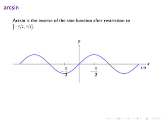
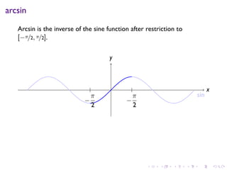
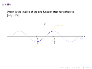
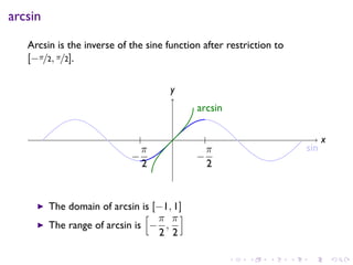
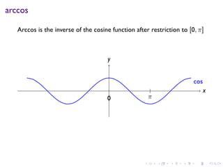
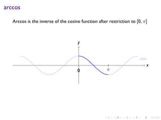
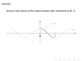
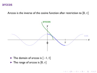
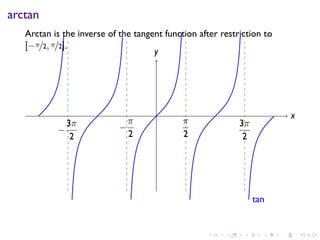
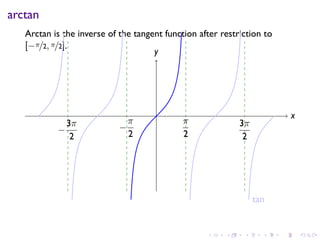
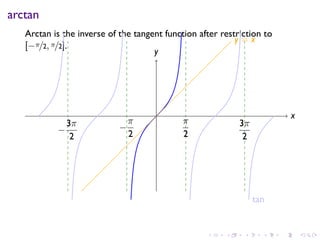
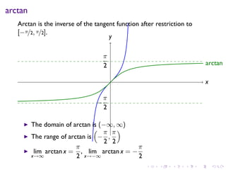
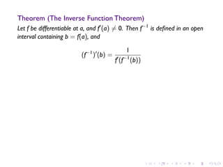
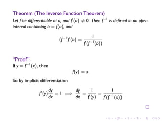
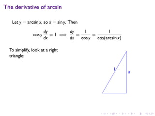
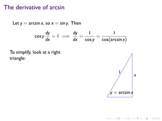
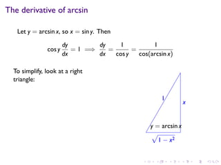
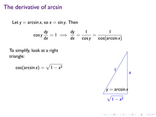
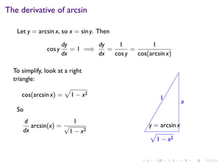
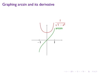
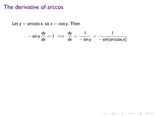
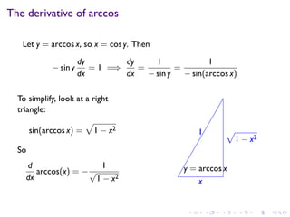
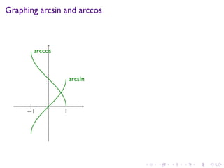
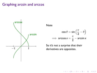
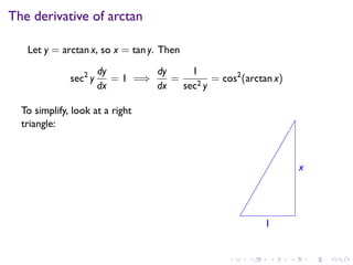
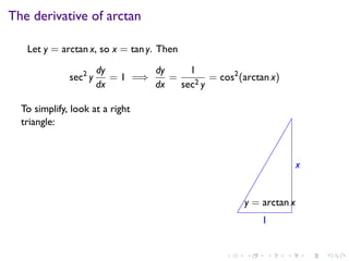
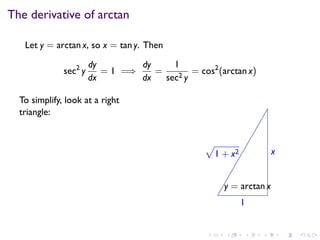
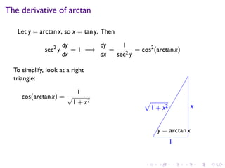
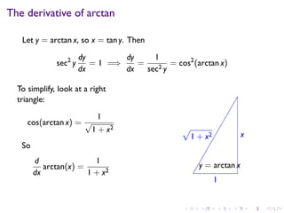
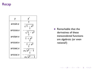
1. The document discusses inverse trigonometric functions such as arcsin, arccos, and arctan.
2. It derives the derivatives of these inverse functions using the Inverse Function Theorem and properties of trigonometric functions.
3. The derivatives are derived to be 1/(√(1-x^2)) for arcsin, 1/√(1-x^2) for arccos, and 1/(1+x^2) for arctan.
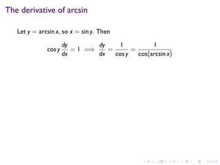
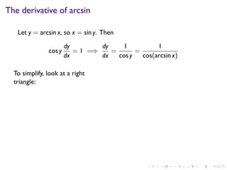
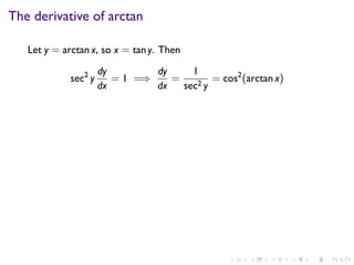
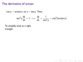
This document summarizes Chapter 10 from a mathematics textbook. The chapter covers limits and continuity. It introduces limits, such as one-sided limits and limits at infinity. It defines continuity as a function being continuous at a point if the limit exists and is equal to the function value. Discontinuities can occur if a limit does not exist or is infinite. The chapter applies limits and continuity to solve inequalities involving polynomials and rational functions. Examples show how to use the definition of a limit to evaluate various types of limits and test continuity.
The document discusses function transformations including shifts, reflections, and stretches/compressions. It defines these transformations and provides examples of how they affect the graph of a function. Specifically, it explains that a shift moves a graph up/down or left/right along an axis, a reflection flips the graph across an axis, and a stretch or compression changes the scale of the graph along an axis. Examples are given of reflecting across the x-axis or y-axis and horizontally or vertically stretching/compressing a function. In the end, students are asked to write equations for specific transformations of a quadratic function.
The document discusses function transformations including translations, reflections, dilations, and compressions. It defines these transformations and provides examples of how they affect the graph of a function. Translations slide the graph left or right without changing its shape or orientation. Reflections create a mirror image of the graph across an axis, flipping it. Compressions squeeze the graph towards or away from an axis. Dilations stretch or shrink the graph away from an axis. The document explains how to interpret various function notation and applies the transformations to example graphs.
1) The document provides an overview of continuity, including defining continuity as a function having a limit equal to its value at a point.
2) It discusses several theorems related to continuity, such as the sum of continuous functions being continuous and various trigonometric, exponential, and logarithmic functions being continuous on their domains.
3) The document also covers inverse trigonometric functions and their domains of continuity.
The document discusses inverse functions, including:
- An inverse function undoes the output of the original function by relating the input and output variables.
- For a function to have an inverse, it must be one-to-one so that each output is paired with a unique input.
- To find the inverse of a function, swap the input and output variables and isolate the new output variable.
We cover the inverses to the trigonometric functions sine, cosine, tangent, cotangent, secant, cosecant, and their derivatives. The remarkable fact is that although these functions and their inverses are transcendental (complicated) functions, the derivatives are algebraic functions. Also, we meet my all-time favorite function: arctan.
This document provides information about inverse functions including:
- The inverse of a function is formed by reversing the coordinates of each ordered pair. A function has an inverse only if it is one-to-one.
- The domain of the inverse function is the range of the original function, and the range of the inverse is the domain of the original.
- To find the inverse of a one-to-one function, replace f(x) with y, interchange x and y, then solve for y in terms of x and replace y with f^-1(x).
- Several examples are provided to demonstrate finding the inverse of different one-to-one functions by following the given steps.
This document discusses integration, which is the inverse process of differentiation. Integration allows us to find the original function given its derivative. Several integration techniques are explained, including substitution, integration by parts, and finding volumes of revolution. Standard integrals are presented along with examples of calculating areas under curves and volumes obtained by rotating areas about axes. Definite integrals are used to find the area between curves over a specified interval.
Increasing and decreasing functions ap calc sec 3.3Ron Eick
The document discusses increasing and decreasing functions and the first derivative test. It defines that a function is increasing if the derivative is positive, decreasing if the derivative is negative, and constant if the derivative is zero. It provides examples of finding the intervals where a function is increasing or decreasing by identifying critical numbers and testing points in each interval. The document also summarizes the first derivative test, stating that a critical point is an extremum if the derivative changes sign there, and whether it is a maximum or minimum depends on if the derivative changes from negative to positive or positive to negative.
1. The document discusses differentiation formulas for hyperbolic functions including sinh, cosh, tanh, coth, sech, and csch. It provides examples of finding the derivatives of functions involving hyperbolic functions.
2. Hyperbolic functions are compared to trigonometric functions, noting that each pair of functions (e.g. sinh and cosh) are inverses of each other. Important hyperbolic identities are also listed.
3. Examples are given of finding the derivatives of functions involving hyperbolic functions, such as f(x) = xsinh(x). The document provides a concise review of differentiation rules for hyperbolic functions and examples of their application.
Using integration by parts, one can evaluate integrals of more complex functions. The formula for integration by parts is:
(u dv - v du) where u and v are the integral and derivative of two functions. Several examples show how to choose u and v and apply the formula repeatedly to simplify integrals. Integration by parts can also be used to evaluate definite integrals using the Fundamental Theorem of Calculus.
The document discusses the chain rule and how to use it to find derivatives of more complex equations. It provides examples of using the chain rule to take derivatives of functions involving exponents, trigonometric functions, radicals, and combinations of these. Key steps include identifying the inner and outer functions, taking the derivative of the inner function, and plugging into the chain rule formula. The document also contrasts using the chain rule method versus the inside-outside method for some problems.
The document summarizes key concepts and applications of integration. It discusses:
1) Important historical figures like Archimedes, Gauss, Leibniz and Newton who contributed to the development of integration and calculus.
2) Engineering applications of integration like in the design of the Petronas Towers and Sydney Opera House.
3) The integration by parts formula and examples of using it to evaluate integrals of composite functions.
This document provides examples and explanations of double integrals. It defines a double integral as integrating a function f(x,y) over a region R in the xy-plane. It then gives three key points:
1) To evaluate a double integral, integrate the inner integral first treating the other variable as a constant, then integrate the outer integral.
2) The easiest regions to integrate over are rectangles, as the limits of integration will all be constants.
3) For non-rectangular regions, the limits of integration may be variable, requiring more careful analysis to determine the limits for each integral.
The document discusses inverse trigonometric functions. It defines the inverse sine function as sin^-1x = arcsin(x), with domain [-1,1] and range [-π/2, π/2]. It provides examples of evaluating inverse trig functions like sin^-1(1/2) = π/6. The inverse cosine function is similarly defined as cos^-1x = arccos(x), with domain [-1,1] and range [0,π]. The document concludes with a short quiz evaluating inverse trig expressions.
This document provides an overview of functions, limits, and continuity. It defines key concepts such as domain and range of functions, and examples of standard real functions. It also covers even and odd functions, and how to calculate limits, including left and right hand limits. Methods for evaluating algebraic limits using substitution, factorization, and rationalization are presented. The objectives are to understand functions, domains, ranges, and how to evaluate limits of functions.
* Recognize graphs of common functions.
* Graph functions using vertical and horizontal shifts.
* Graph functions using reflections about the x-axis and the y-axis.
* Graph functions using compressions and stretches.
* Combine transformations.
Complex numbers are numbers of the form a + bi, where a is the real part and bi is the imaginary part. Complex numbers can be added, subtracted, multiplied, and divided. When multiplying complex numbers, the real parts and imaginary parts are multiplied separately and combined. The conjugate of a + bi is a - bi. When a complex number is multiplied by its conjugate, the result is a real number equal to the modulus (magnitude) of the complex number squared. Complex numbers can also be expressed in polar form as r(cosθ + i sinθ), where r is the modulus and θ is the argument.
This document discusses trigonometric functions and identities. It provides definitions of trig functions like sine, cosine, tangent, and cotangent. It then lists 8 fundamental trigonometric identities and the reciprocal, quotient, and Pythagorean relations between trig functions. It gives conditions and rules for transforming trig identities and examples of proving identities like secθ cotθ = cscθ and 2cos2θ - 1 = cos2θ−sin2θ. The document assigns proving additional identities like secѲ/cscѲ = tanѲ as homework.
This chapter discusses differentiation, including:
- Defining the derivative using the limit definition of the slope of a tangent line.
- Basic differentiation rules for constants, polynomials, sums and differences.
- Interpreting the derivative as an instantaneous rate of change.
- Applying the product rule and quotient rule to differentiate products and quotients.
- Using differentiation to find equations of tangent lines, velocities, marginal costs, and other rates of change.
This document provides an overview of Chapter 3 from a Calculus I course on derivatives. It introduces the concept of the derivative and how it relates to tangent lines and rates of change. The chapter outline describes sections on the derivative of functions, rules of derivatives, derivatives of trigonometric functions, the chain rule, and implicit differentiation. Examples are provided for taking derivatives of various functions, including constant functions, power functions, sums and differences, and products. Higher derivatives are also introduced.
The document discusses different types of functions and their graphs. It provides examples of constant functions, linear functions, quadratic functions, and absolute value functions. It shows how to graph each type of function by plotting points and describes their domains and ranges. For linear functions, the domain is all real numbers and the range is also all real numbers. For quadratic functions, the graph is a parabola and the range only includes positive values. Absolute value functions have a domain of all real numbers and a range that is positive and excludes negative values below the constant.
Lesson3.1 The Derivative And The Tangent Lineseltzermath
This document provides an introduction to the concept of the tangent line and derivative. It defines the tangent line as the line that intersects a curve at exactly one point. It discusses how to approximate the slope of a tangent line using secant lines and taking the limit as the second point approaches the point of tangency. The derivative is defined as the formula that gives the slope of the tangent line at any point on a curve. It provides examples of using calculators to calculate derivatives and discusses how the graph of a derivative relates to properties of the original function such as maxima, minima and x-intercepts.
L19 increasing & decreasing functionsJames Tagara
This document discusses analysis of functions including derivatives, extrema, and graphing. It defines key concepts such as increasing and decreasing functions, concavity, points of inflection, stationary points, and relative maxima and minima. It presents Rolle's theorem and the mean value theorem. Examples demonstrate finding critical points and determining the behavior of functions based on the signs of the first and second derivatives. The first and second derivative tests are introduced to identify relative extrema at critical points.
The document defines complex numbers and their properties. It states that a complex number has the form x + iy, where x and y are real numbers and i = √-1. Complex numbers can be represented in rectangular form as x + iy or in polar form as r(cosθ + i sinθ), where r is the modulus or absolute value and θ is the argument. The document also defines conjugate complex numbers and describes how to calculate the sum, difference, and product of two complex numbers.
This document defines and provides examples of the domain and range of a function. The domain is the set of all independent variable (x-coordinate) values, while the range is the set of all dependent variable (y-coordinate) values. Several examples of identifying the domain and range of functions given their sets of ordered pairs are provided. The document also discusses using the vertical line test to determine if a graph represents a function.
The document summarizes the key properties and graphs of six trigonometric functions: sine, cosine, tangent, cotangent, secant, and cosecant. For each function, it discusses amplitude, period, zeros or asymptotes, and shows an example graph over one period. It also covers transformations of trig functions that change amplitude, period, phase and vertical shifts.
The document discusses inverse functions, logarithmic functions, and their properties. It defines an inverse function f^-1(x) as satisfying f(f^-1(x)) = x. It also defines the logarithm log_a(x) as the inverse of the exponential function a^x. Key properties of inverse functions and logarithms are outlined, including: the derivative of an inverse function using the inverse function theorem; logarithm rules such as log_a(xy) = log_a(x) + log_a(y); and converting between logarithmic bases using ln(x)/ln(a). Examples of evaluating and graphing inverse functions and logarithms are provided.
The document appears to be lecture slides for a Calculus I class at NYU. It discusses announcements like midterm grades being submitted and an upcoming quiz. It then summarizes student evaluations of the class, including both positive and negative feedback. The remainder of the document outlines and discusses the topics of inverse trigonometric functions, including their definitions, domains, ranges, and derivatives. Graphs are provided to illustrate inverse functions and how to obtain the graph of an inverse from the original function. Specific inverse trig functions like arcsin and arccos are defined.
This document contains lecture notes on inverse trigonometric functions. It begins with definitions of inverse functions and conditions for a function to have an inverse. It then defines the inverse trigonometric functions arcsin, arccos, arctan, and arcsec and gives their domains and ranges. Examples are provided to illustrate calculating values of the inverse trigonometric functions. The document concludes with a brief discussion of notational ambiguity and an outline mentioning derivatives of inverse trigonometric functions and applications.
This document contains information about trigonometric ratios including:
- Definitions of sine, cosine, tangent, cotangent, secant, and cosecant ratios in terms of right triangles.
- Graphs of the trigonometric ratios over one period.
- Properties of trigonometric ratios including relationships between ratios and values for special angles like 0, 30, 45, 60, 90 degrees.
- Operations with trigonometric ratios including inverting ratios and dealing with negative angles.
- Identifying ratios in different quadrants based on signs.
- Solving trigonometric equations using identities.
The document discusses trigonometric functions and right triangles. It defines the six trigonometric functions as ratios between pairs of sides in a right triangle. The first three functions are sine, cosine, and tangent, which relate the opposite, adjacent, and hypotenuse sides to a given angle. The other three are the reciprocals of the first three and complete the set of basic trigonometric functions.
The document discusses trigonometric ratios and functions. It provides information on:
1) Trigonometric ratios in the four quadrants and for angles greater than 360 degrees, including how the ratios change based on the quadrant or whether the angle is an even or odd multiple of 90 degrees.
2) How to solve trigonometric equations involving sin, cos, and tan, including using identities and periodicity.
3) How to draw and analyze simple graphs of the trigonometric functions sin x, cos x, and tan x, including finding intercepts and maximum/minimum values.
1) The document defines and discusses the domains and ranges of inverse trigonometric functions such as sin-1x, cos-1x, and tan-1x.
2) The inverse functions are defined based on reflecting portions of the original trigonometric functions over the line y=x.
3) The domains and ranges of the inverse functions are restricted to ensure each inverse function is a single-valued function.
We define what it means for a function to have a maximum or minimum value, and explain the Extreme Value Theorem, which indicates these maxima and minima must be there under certain conditions.
Fermat's Theorem says that at differentiable extreme points, the derivative should be zero, and thus we arrive at a technique for finding extrema: look among the endpoints of the domain of definition and the critical points of the function.
There's also a little digression on Fermat's Last theorem, which is not related to calculus but is a big deal in recent mathematical history.
This document discusses limits involving infinity in calculus. It begins with definitions of infinite limits, both positive and negative infinity. It provides examples of common infinite limits, such as the limit of 1/x as x approaches 0. It also discusses vertical asymptotes and rules for infinite limits, such as the limit of a sum being infinity if both terms have infinite limits. The document contains examples evaluating limits at points where functions are not continuous.
This document discusses finding the maximum and minimum values of functions. It introduces the Extreme Value Theorem, which states that if a function is continuous on a closed interval, then it attains both a maximum and minimum value on that interval. It also discusses Fermat's Theorem, which relates local extrema of a differentiable function to its derivative. Examples are provided to illustrate these concepts.
The document discusses the chain rule for calculating the derivative of composite functions. It states that if a function F is composed of two differentiable functions g and φ, where F(x) = φ(g(x)), then F is differentiable and its derivative can be found using the chain rule. It asks the reader to identify the inner and outer functions for examples of composite functions.
The document discusses functions and their inverse functions. It provides an analogy that functions are like dye that colors eggs, and the inverse "undoes" the dye by bleaching the egg. The inverse of a function undoes what the original function did. For the square function f(x)=x^2, its inverse is the square root function. Graphically, the inverse function switches the x and y values of a point. The graphs of a function and its inverse are mirror images across the line y=x. Examples are provided to demonstrate finding the inverse of functions by switching x and y and solving for y.
Using the Mean Value Theorem, we can show the a function is increasing on an interval when its derivative is positive on the interval. Changes in the sign of the derivative detect local extrema. We also can use the second derivative to detect concavity and inflection points. This means that the first and second derivative can be used to classify critical points as local maxima or minima
1. The document discusses the chain rule for finding the derivative of a composition of two functions f and g.
2. The chain rule states that the derivative of the composition f(g(x)) is the product of the derivative of the outer function f evaluated at g(x) and the derivative of the inner function g.
3. An example using linear functions shows that the derivative of a composition of two linear functions results in another linear function whose slope is the product of the original slopes.
This document provides guidance on developing effective lesson plans for calculus instructors. It recommends starting by defining specific learning objectives and assessments. Examples should be chosen carefully to illustrate concepts and engage students at a variety of levels. The lesson plan should include an introductory problem, definitions, theorems, examples, and group work. Timing for each section should be estimated. After teaching, the lesson can be improved by analyzing what was effective and what needs adjustment for the next time. Advanced preparation is key to looking prepared and ensuring students learn.
Streamlining assessment, feedback, and archival with auto-multiple-choiceMatthew Leingang
Auto-multiple-choice (AMC) is an open-source optical mark recognition software package built with Perl, LaTeX, XML, and sqlite. I use it for all my in-class quizzes and exams. Unique papers are created for each student, fixed-response items are scored automatically, and free-response problems, after manual scoring, have marks recorded in the same process. In the first part of the talk I will discuss AMC’s many features and why I feel it’s ideal for a mathematics course. My contributions to the AMC workflow include some scripts designed to automate the process of returning scored papers
back to students electronically. AMC provides an email gateway, but I have written programs to return graded papers via the DAV protocol to student’s dropboxes on our (Sakai) learning management systems. I will also show how graded papers can be archived, with appropriate metadata tags, into an Evernote notebook.
This document discusses electronic grading of paper assessments using PDF forms. Key points include:
- Various tools for creating fillable PDF forms using LaTeX packages or desktop software.
- Methods for stamping completed forms onto scanned documents including using pdftk or overlaying in TikZ.
- Options for grading on tablets or desktops including GoodReader, PDFExpert, Adobe Acrobat.
- Extracting data from completed forms can be done in Adobe Acrobat or via command line with pdftk.
Integration by substitution is the chain rule in reverse.
NOTE: the final location is section specific. Section 1 (morning) is in SILV 703, Section 11 (afternoon) is in CANT 200
Lesson 26: The Fundamental Theorem of Calculus (slides)Matthew Leingang
g(x) represents the area under the curve of f(t) between 0 and x.
.
x
What can you say about g? 2 4 6 8 10f
The First Fundamental Theorem of Calculus
Theorem (First Fundamental Theorem of Calculus)
Let f be a con nuous func on on [a, b]. Define the func on F on [a, b] by
∫ x
F(x) = f(t) dt
a
Then F is con nuous on [a, b] and differentiable on (a, b) and for all x in (a, b),
F′(x
Lesson 26: The Fundamental Theorem of Calculus (slides)Matthew Leingang
The document discusses the Fundamental Theorem of Calculus, which has two parts. The first part states that if a function f is continuous on an interval, then the derivative of the integral of f is equal to f. This is proven using Riemann sums. The second part relates the integral of a function f to the integral of its derivative F'. Examples are provided to illustrate how the area under a curve relates to these concepts.
Lesson 27: Integration by Substitution (handout)Matthew Leingang
This document contains lecture notes on integration by substitution from a Calculus I class. It introduces the technique of substitution for both indefinite and definite integrals. For indefinite integrals, the substitution rule is presented, along with examples of using substitutions to evaluate integrals involving polynomials, trigonometric, exponential, and other functions. For definite integrals, the substitution rule is extended and examples are worked through both with and without first finding the indefinite integral. The document emphasizes that substitution often simplifies integrals and makes them easier to evaluate.
Lesson 26: The Fundamental Theorem of Calculus (handout)Matthew Leingang
1) The document discusses lecture notes on Section 5.4: The Fundamental Theorem of Calculus from a Calculus I course. 2) It covers stating and explaining the Fundamental Theorems of Calculus and using the first fundamental theorem to find derivatives of functions defined by integrals. 3) The lecture outlines the first fundamental theorem, which relates differentiation and integration, and gives examples of applying it.
This document contains notes from a calculus class lecture on evaluating definite integrals. It discusses using the evaluation theorem to evaluate definite integrals, writing derivatives as indefinite integrals, and interpreting definite integrals as the net change of a function over an interval. The document also contains examples of evaluating definite integrals, properties of integrals, and an outline of the key topics covered.
This document contains lecture notes from a Calculus I class covering Section 5.3 on evaluating definite integrals. The notes discuss using the Evaluation Theorem to calculate definite integrals, writing derivatives as indefinite integrals, and interpreting definite integrals as the net change of a function over an interval. Examples are provided to demonstrate evaluating definite integrals using the midpoint rule approximation. Properties of integrals such as additivity and the relationship between definite and indefinite integrals are also outlined.
Lesson 24: Areas and Distances, The Definite Integral (handout)Matthew Leingang
We can define the area of a curved region by a process similar to that by which we determined the slope of a curve: approximation by what we know and a limit.
Lesson 24: Areas and Distances, The Definite Integral (slides)Matthew Leingang
We can define the area of a curved region by a process similar to that by which we determined the slope of a curve: approximation by what we know and a limit.
At times it is useful to consider a function whose derivative is a given function. We look at the general idea of reversing the differentiation process and its applications to rectilinear motion.
This document contains lecture notes from a Calculus I class discussing optimization problems. It begins with announcements about upcoming exams and courses the professor is teaching. It then presents an example problem about finding the rectangle of a fixed perimeter with the maximum area. The solution uses calculus techniques like taking the derivative to find the critical points and determine that the optimal rectangle is a square. The notes discuss strategies for solving optimization problems and summarize the key steps to take.
Uncountably many problems in life and nature can be expressed in terms of an optimization principle. We look at the process and find a few good examples.
The document discusses curve sketching of functions by analyzing their derivatives. It provides:
1) A checklist for graphing a function which involves finding where the function is positive/negative/zero, its monotonicity from the first derivative, and concavity from the second derivative.
2) An example of graphing the cubic function f(x) = 2x^3 - 3x^2 - 12x through analyzing its derivatives.
3) Explanations of the increasing/decreasing test and concavity test to determine monotonicity and concavity from a function's derivatives.
The document contains lecture notes on curve sketching from a Calculus I class. It discusses using the first and second derivative tests to determine properties of a function like monotonicity, concavity, maxima, minima, and points of inflection in order to sketch the graph of the function. It then provides an example of using these tests to sketch the graph of the cubic function f(x) = 2x^3 - 3x^2 - 12x.
Lesson 20: Derivatives and the Shapes of Curves (slides)Matthew Leingang
This document contains lecture notes on derivatives and the shapes of curves from a Calculus I class taught by Professor Matthew Leingang at New York University. The notes cover using derivatives to determine the intervals where a function is increasing or decreasing, classifying critical points as maxima or minima, using the second derivative to determine concavity, and applying the first and second derivative tests. Examples are provided to illustrate finding intervals of monotonicity for various functions.
Lesson 20: Derivatives and the Shapes of Curves (handout)Matthew Leingang
This document contains lecture notes on calculus from a Calculus I course. It covers determining the monotonicity of functions using the first derivative test. Key points include using the sign of the derivative to determine if a function is increasing or decreasing over an interval, and using the first derivative test to classify critical points as local maxima, minima, or neither. Examples are provided to demonstrate finding intervals of monotonicity for various functions and applying the first derivative test.
How to Fix the Import Error in the Odoo 17Celine George
An import error occurs when a program fails to import a module or library, disrupting its execution. In languages like Python, this issue arises when the specified module cannot be found or accessed, hindering the program's functionality. Resolving import errors is crucial for maintaining smooth software operation and uninterrupted development processes.
A Strategic Approach: GenAI in EducationPeter Windle
Artificial Intelligence (AI) technologies such as Generative AI, Image Generators and Large Language Models have had a dramatic impact on teaching, learning and assessment over the past 18 months. The most immediate threat AI posed was to Academic Integrity with Higher Education Institutes (HEIs) focusing their efforts on combating the use of GenAI in assessment. Guidelines were developed for staff and students, policies put in place too. Innovative educators have forged paths in the use of Generative AI for teaching, learning and assessments leading to pockets of transformation springing up across HEIs, often with little or no top-down guidance, support or direction.
This Gasta posits a strategic approach to integrating AI into HEIs to prepare staff, students and the curriculum for an evolving world and workplace. We will highlight the advantages of working with these technologies beyond the realm of teaching, learning and assessment by considering prompt engineering skills, industry impact, curriculum changes, and the need for staff upskilling. In contrast, not engaging strategically with Generative AI poses risks, including falling behind peers, missed opportunities and failing to ensure our graduates remain employable. The rapid evolution of AI technologies necessitates a proactive and strategic approach if we are to remain relevant.
हिंदी वर्णमाला पीपीटी, hindi alphabet PPT presentation, hindi varnamala PPT, Hindi Varnamala pdf, हिंदी स्वर, हिंदी व्यंजन, sikhiye hindi varnmala, dr. mulla adam ali, hindi language and literature, hindi alphabet with drawing, hindi alphabet pdf, hindi varnamala for childrens, hindi language, hindi varnamala practice for kids, https://www.drmullaadamali.com
Macroeconomics- Movie Location
This will be used as part of your Personal Professional Portfolio once graded.
Objective:
Prepare a presentation or a paper using research, basic comparative analysis, data organization and application of economic information. You will make an informed assessment of an economic climate outside of the United States to accomplish an entertainment industry objective.
How to Manage Your Lost Opportunities in Odoo 17 CRMCeline George
Odoo 17 CRM allows us to track why we lose sales opportunities with "Lost Reasons." This helps analyze our sales process and identify areas for improvement. Here's how to configure lost reasons in Odoo 17 CRM
This presentation includes basic of PCOS their pathology and treatment and also Ayurveda correlation of PCOS and Ayurvedic line of treatment mentioned in classics.
it describes the bony anatomy including the femoral head , acetabulum, labrum . also discusses the capsule , ligaments . muscle that act on the hip joint and the range of motion are outlined. factors affecting hip joint stability and weight transmission through the joint are summarized.
How to Add Chatter in the odoo 17 ERP ModuleCeline George
In Odoo, the chatter is like a chat tool that helps you work together on records. You can leave notes and track things, making it easier to talk with your team and partners. Inside chatter, all communication history, activity, and changes will be displayed.
1. Section 3.5
Inverse Trigonometric
Functions
V63.0121, Calculus I
March 11–12, 2009
Announcements
Get half of your unearned ALEKS points back by March 22
. . . . . .
2. What functions are invertible?
In order for f−1 to be a function, there must be only one a in D
corresponding to each b in E.
Such a function is called one-to-one
The graph of such a function passes the horizontal line test:
any horizontal line intersects the graph in exactly one point if at
all.
If f is continuous, then f−1 is continuous.
. . . . . .
4. arcsin
Arcsin is the inverse of the sine function after restriction to
[−π/2, π/2].
y
.
. . . x
.
s
. in
π π
− −
. .
2 2
. . . . . .
5. arcsin
Arcsin is the inverse of the sine function after restriction to
[−π/2, π/2].
y
.
. . . x
.
s
. in
π π
− −
. .
2 2
. . . . . .
6. arcsin
Arcsin is the inverse of the sine function after restriction to
[−π/2, π/2].
y
.
. =x
y
. . . x
.
s
. in
π π
− −
. .
2 2
. . . . . .
7. arcsin
Arcsin is the inverse of the sine function after restriction to
[−π/2, π/2].
y
.
a
. rcsin
. . . x
.
s
. in
π π
− −
. .
2 2
The domain of arcsin is [−1, 1]
[ π π]
The range of arcsin is − ,
22
. . . . . .
8. arccos
Arccos is the inverse of the cosine function after restriction to [0, π]
y
.
c
. os
. . x
.
π
.
0
.
. . . . . .
9. arccos
Arccos is the inverse of the cosine function after restriction to [0, π]
y
.
c
. os
. . x
.
π
.
0
.
. . . . . .
10. arccos
Arccos is the inverse of the cosine function after restriction to [0, π]
y
.
. =x
y
c
. os
. . x
.
π
.
0
.
. . . . . .
11. arccos
Arccos is the inverse of the cosine function after restriction to [0, π]
a
. rccos
y
.
c
. os
. . x
.
π
.
0
.
The domain of arccos is [−1, 1]
The range of arccos is [0, π]
. . . . . .
12. arctan
Arctan is the inverse of the tangent function after restriction to
[−π/2, π/2].
y
.
. x
.
π π
3π 3π
−
− . .
. .
2 2
2 2
t
. an
. . . . . .
13. arctan
Arctan is the inverse of the tangent function after restriction to
[−π/2, π/2].
y
.
. x
.
π π
3π 3π
−
− . .
. .
2 2
2 2
t
. an
. . . . . .
14. arctan
Arctan is the inverse of the tangent function after restriction to
. =x
y
[−π/2, π/2].
y
.
. x
.
π π
3π 3π
−
− . .
. .
2 2
2 2
t
. an
. . . . . .
15. arctan
Arctan is the inverse of the tangent function after restriction to
[−π/2, π/2].
y
.
π
. a
. rctan
2
. x
.
π
−
.
2
The domain of arctan is (−∞, ∞)
( π π)
The range of arctan is − ,
22
π π
lim arctan x = , lim arctan x = −
2 x→−∞ 2
x→∞
. . . . . .
17. Theorem (The Inverse Function Theorem)
Let f be differentiable at a, and f′ (a) ̸= 0. Then f−1 is defined in an open
interval containing b = f(a), and
1
(f−1 )′ (b) = ′ −1
f (f (b))
. . . . . .
18. Theorem (The Inverse Function Theorem)
Let f be differentiable at a, and f′ (a) ̸= 0. Then f−1 is defined in an open
interval containing b = f(a), and
1
(f−1 )′ (b) = ′ −1
f (f (b))
“Proof”.
If y = f−1 (x), then
f(y) = x,
So by implicit differentiation
dy dy 1 1
f′ (y) = 1 =⇒ =′ = ′ −1
dx dx f (y) f (f (x))
. . . . . .
19. The derivative of arcsin
Let y = arcsin x, so x = sin y. Then
dy dy 1 1
= 1 =⇒ = =
cos y
dx dx cos y cos(arcsin x)
. . . . . .
20. The derivative of arcsin
Let y = arcsin x, so x = sin y. Then
dy dy 1 1
= 1 =⇒ = =
cos y
dx dx cos y cos(arcsin x)
To simplify, look at a right
triangle:
.
. . . . . .
21. The derivative of arcsin
Let y = arcsin x, so x = sin y. Then
dy dy 1 1
= 1 =⇒ = =
cos y
dx dx cos y cos(arcsin x)
To simplify, look at a right
triangle:
1
.
x
.
.
. . . . . .
22. The derivative of arcsin
Let y = arcsin x, so x = sin y. Then
dy dy 1 1
= 1 =⇒ = =
cos y
dx dx cos y cos(arcsin x)
To simplify, look at a right
triangle:
1
.
x
.
. = arcsin x
y
.
. . . . . .
23. The derivative of arcsin
Let y = arcsin x, so x = sin y. Then
dy dy 1 1
= 1 =⇒ = =
cos y
dx dx cos y cos(arcsin x)
To simplify, look at a right
triangle:
1
.
x
.
. = arcsin x
y
.√
. 1 − x2
. . . . . .
24. The derivative of arcsin
Let y = arcsin x, so x = sin y. Then
dy dy 1 1
= 1 =⇒ = =
cos y
dx dx cos y cos(arcsin x)
To simplify, look at a right
triangle:
√
cos(arcsin x) = 1 − x2 1
.
x
.
. = arcsin x
y
.√
. 1 − x2
. . . . . .
25. The derivative of arcsin
Let y = arcsin x, so x = sin y. Then
dy dy 1 1
= 1 =⇒ = =
cos y
dx dx cos y cos(arcsin x)
To simplify, look at a right
triangle:
√
cos(arcsin x) = 1 − x2 1
.
x
.
So
d 1
arcsin(x) = √ . = arcsin x
y
1 − x2 .√
dx
. 1 − x2
. . . . . .
26. Graphing arcsin and its derivative
1
.√
1 − x2
a
. rcsin
.
| |
. .
−
.1 1
.
. . . . . .
27. The derivative of arccos
Let y = arccos x, so x = cos y. Then
dy dy 1 1
− sin y = 1 =⇒ = =
− sin y − sin(arccos x)
dx dx
. . . . . .
28. The derivative of arccos
Let y = arccos x, so x = cos y. Then
dy dy 1 1
− sin y = 1 =⇒ = =
− sin y − sin(arccos x)
dx dx
To simplify, look at a right
triangle:
√
sin(arccos x) = 1 − x2 √
1
.
. 1 − x2
So
d 1 . = arccos x
y
arccos(x) = − √ .
1 − x2
dx x
.
. . . . . .
29. Graphing arcsin and arccos
a
. rccos
a
. rcsin
.
| |
. .
−
.1 1
.
. . . . . .
30. Graphing arcsin and arccos
a
. rccos
Note
(π )
−θ
cos θ = sin
2
a
. rcsin
π
=⇒ arccos x = − arcsin x
2
. So it’s not a surprise that their
| |
. .
−
.1 1
. derivatives are opposites.
. . . . . .
31. The derivative of arctan
Let y = arctan x, so x = tan y. Then
dy dy 1
sec2 y = cos2 (arctan x)
= 1 =⇒ =
sec2 y
dx dx
. . . . . .
32. The derivative of arctan
Let y = arctan x, so x = tan y. Then
dy dy 1
sec2 y = cos2 (arctan x)
= 1 =⇒ =
sec2 y
dx dx
To simplify, look at a right
triangle:
.
. . . . . .
33. The derivative of arctan
Let y = arctan x, so x = tan y. Then
dy dy 1
sec2 y = cos2 (arctan x)
= 1 =⇒ =
sec2 y
dx dx
To simplify, look at a right
triangle:
x
.
.
1
.
. . . . . .
34. The derivative of arctan
Let y = arctan x, so x = tan y. Then
dy dy 1
sec2 y = cos2 (arctan x)
= 1 =⇒ =
sec2 y
dx dx
To simplify, look at a right
triangle:
x
.
. = arctan x
y
.
1
.
. . . . . .
35. The derivative of arctan
Let y = arctan x, so x = tan y. Then
dy dy 1
sec2 y = cos2 (arctan x)
= 1 =⇒ =
sec2 y
dx dx
To simplify, look at a right
triangle:
√
x
.
. 1 + x2
. = arctan x
y
.
1
.
. . . . . .
36. The derivative of arctan
Let y = arctan x, so x = tan y. Then
dy dy 1
sec2 y = cos2 (arctan x)
= 1 =⇒ =
sec2 y
dx dx
To simplify, look at a right
triangle:
1
cos(arctan x) = √
√
1 + x2
x
.
. 1 + x2
. = arctan x
y
.
1
.
. . . . . .
37. The derivative of arctan
Let y = arctan x, so x = tan y. Then
dy dy 1
sec2 y = cos2 (arctan x)
= 1 =⇒ =
sec2 y
dx dx
To simplify, look at a right
triangle:
1
cos(arctan x) = √
√
1 + x2
x
.
. 1 + x2
So
d 1
. = arctan x
y
arctan(x) =
.
1 + x2
dx
1
.
. . . . . .
39. Example
√
x. Find f′ (x).
Let f(x) = arctan
. . . . . .
40. Example
√
x. Find f′ (x).
Let f(x) = arctan
Solution
√ d√
d 1 1 1
·√
(√ )2
arctan x = x=
1+x 2 x
dx x dx
1+
1
=√ √
2 x + 2x x
. . . . . .
41. Recap
y′
y
1
√
arcsin x
1 − x2
1 Remarkable that the
arccos x − √
1 − x2 derivatives of these
1 transcendental functions
arctan x
1 + x2 are algebraic (or even
1
−
arccot x rational!)
1 + x2
1
√
arcsec x
x x2 − 1
1
arccsc x − √
x x2 − 1
. . . . . .