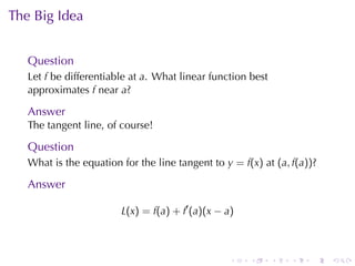
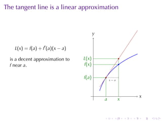
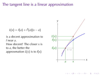
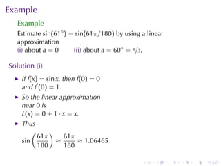
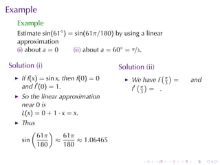
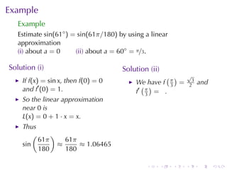
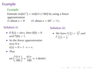
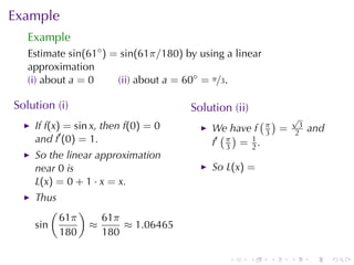
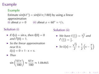
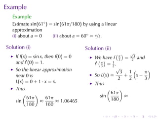
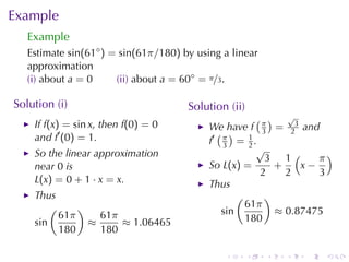
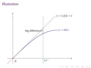
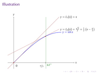
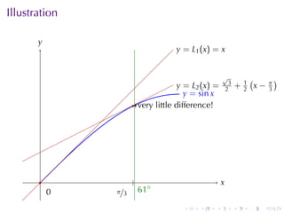
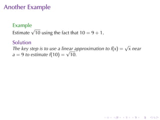
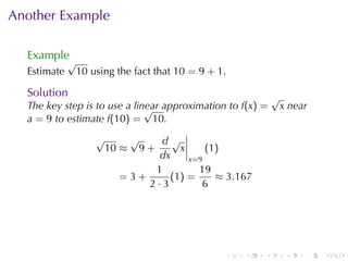
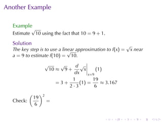
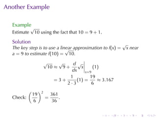
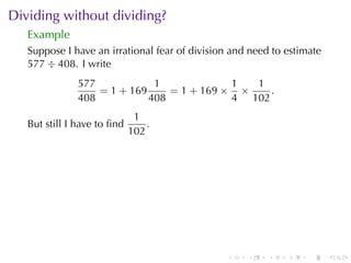
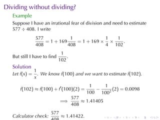
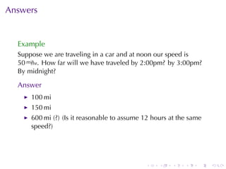
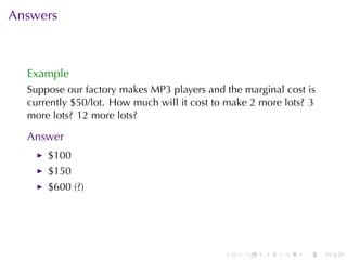
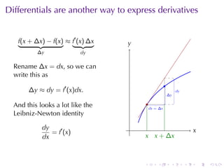
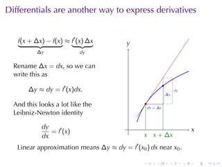
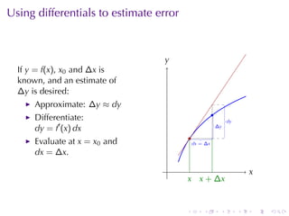
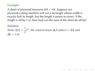
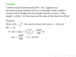
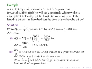
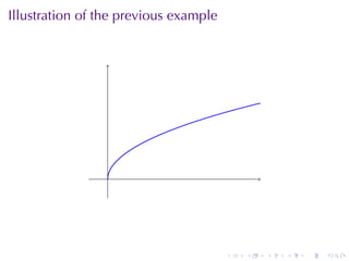
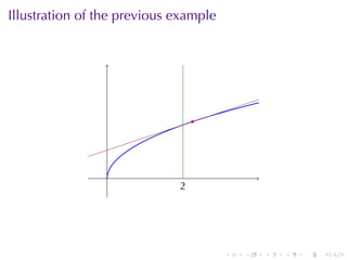
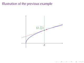
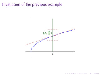
The tangent line to the graph of a function at a point is the best linear function which agrees with the given function at the point. The function and its linear approximation will probably diverge away from the point at which they agree, but this "error" can be measured using the differential notation.
Lesson 12: Linear Approximation and DifferentialsMatthew Leingang
ย
The tangent line to the graph of a function at a point can be thought of as a function itself. As such, it is the best linear function which agrees with the given function at the point. The function and its linear approximation will probably diverge away from the point at which they agree, but this "error" can be measured using the differential notation.
Lesson 12: Linear Approximations and Differentials (slides)Matthew Leingang
ย
The line tangent to a curve is also the line which best "fits" the curve near that point. So derivatives can be used for approximating complicated functions with simple linear ones. Differentials are another set of notation for the same problem.
From moments to sparse representations, a geometric, algebraic and algorithmi...BernardMourrain
ย
Tensors (10-14 September 2018, Polytechnico di Torino) - From moments to sparse representations, a geometric, algebraic and algorithmic viewpoint. Tensors (10-14 September 2018, Polytechnico di Torino) - From moments to sparse representations, a geometric, algebraic and algorithmic viewpoint. Part 1.
Lesson 13: Exponential and Logarithmic Functions (slides)Matthew Leingang
ย
The document provides an outline and definitions for sections 3.1 and 3.2 of a calculus class, which cover exponential and logarithmic functions. It defines exponential functions, establishes conventions for exponents of all types, and graphs exponential functions. Key points covered include the properties of exponential functions and defining exponents for non-whole number bases.
Lesson 14: Derivatives of Logarithmic and Exponential Functions (slides)Matthew Leingang
ย
The exponential function is pretty much the only function whose derivative is itself. The derivative of the natural logarithm function is also beautiful as it fills in an important gap. Finally, the technique of logarithmic differentiation allows us to find derivatives without the product rule.
Lesson 20: Derivatives and the Shapes of Curves (slides)Matthew Leingang
ย
This document contains lecture notes on derivatives and the shapes of curves from a Calculus I class taught by Professor Matthew Leingang at New York University. The notes cover using derivatives to determine the intervals where a function is increasing or decreasing, classifying critical points as maxima or minima, using the second derivative to determine concavity, and applying the first and second derivative tests. Examples are provided to illustrate finding intervals of monotonicity for various functions.
Lesson 12: Linear Approximation and DifferentialsMatthew Leingang
ย
The tangent line to the graph of a function at a point can be thought of as a function itself. As such, it is the best linear function which agrees with the given function at the point. The function and its linear approximation will probably diverge away from the point at which they agree, but this "error" can be measured using the differential notation.
Lesson 12: Linear Approximations and Differentials (slides)Matthew Leingang
ย
The line tangent to a curve is also the line which best "fits" the curve near that point. So derivatives can be used for approximating complicated functions with simple linear ones. Differentials are another set of notation for the same problem.
From moments to sparse representations, a geometric, algebraic and algorithmi...BernardMourrain
ย
Tensors (10-14 September 2018, Polytechnico di Torino) - From moments to sparse representations, a geometric, algebraic and algorithmic viewpoint. Tensors (10-14 September 2018, Polytechnico di Torino) - From moments to sparse representations, a geometric, algebraic and algorithmic viewpoint. Part 1.
Lesson 13: Exponential and Logarithmic Functions (slides)Matthew Leingang
ย
The document provides an outline and definitions for sections 3.1 and 3.2 of a calculus class, which cover exponential and logarithmic functions. It defines exponential functions, establishes conventions for exponents of all types, and graphs exponential functions. Key points covered include the properties of exponential functions and defining exponents for non-whole number bases.
Lesson 14: Derivatives of Logarithmic and Exponential Functions (slides)Matthew Leingang
ย
The exponential function is pretty much the only function whose derivative is itself. The derivative of the natural logarithm function is also beautiful as it fills in an important gap. Finally, the technique of logarithmic differentiation allows us to find derivatives without the product rule.
Lesson 20: Derivatives and the Shapes of Curves (slides)Matthew Leingang
ย
This document contains lecture notes on derivatives and the shapes of curves from a Calculus I class taught by Professor Matthew Leingang at New York University. The notes cover using derivatives to determine the intervals where a function is increasing or decreasing, classifying critical points as maxima or minima, using the second derivative to determine concavity, and applying the first and second derivative tests. Examples are provided to illustrate finding intervals of monotonicity for various functions.
The simplex algorithm is used to solve linear programming problems by iteratively moving from one basic feasible solution (BFS) to another with a better objective value. It starts at an initial BFS and checks if it is optimal. If not, it moves to a new improved BFS and repeats the process until an optimal solution is found. For the example problem of maximizing profit from two drugs given machine time constraints, the algorithm starts at BFS (0,0,9,8) and improves to BFS (4,0,5,0) by increasing the variable with the largest coefficient in the objective function while maintaining feasibility.
At times it is useful to consider a function whose derivative is a given function. We look at the general idea of reversing the differentiation process and its applications to rectilinear motion.
This document discusses two applications of tangent lines: differentials and linear approximation, and finding the tangent line T(b) at a nearby point b. It explains that the tangent line T(x) at point (a, f(a)) is given by T(x) = f'(a)(x - a) + f(a). The slope f'(a) is identified with the derivative dy/dx. There are two ways to find T(b): directly using T(x), or by finding the differential ฮT = dy and using ฮT + f(a) = T(b).
1. This document provides step-by-step instructions for solving various calculus problems including finding zeros, derivatives, integrals, limits, continuity, asymptotes, extrema, and solving differential equations.
2. For each type of problem, it lists the key steps to take in a "You think..." prompt followed by more detailed explanations and formulas.
3. The document is intended as a reference for a student to know the general approach and techniques for multiple calculus problems at a glance.
This document discusses the concept of the derivative and differentiation. It begins by explaining how the slope of a curve changes at different points, unlike the constant slope of a line. It then defines the derivative of a function f at a point x0 as the limit of the difference quotient as h approaches 0. If this limit exists, then f is said to be differentiable at x0. The derivative f'(x) then represents the slope of the curve y=f(x) at each point x and is a measure of how steeply the curve is rising or falling at that point. Several examples are provided to illustrate how to compute derivatives using this limit definition.
Lesson 15: Exponential Growth and Decay (slides)Matthew Leingang
ย
Many problems in nature are expressible in terms of a certain differential equation that has a solution in terms of exponential functions. We look at the equation in general and some fun applications, including radioactivity, cooling, and interest.
1) The document provides an overview of continuity, including defining continuity as a function having a limit equal to its value at a point.
2) It discusses several theorems related to continuity, such as the sum of continuous functions being continuous and various trigonometric, exponential, and logarithmic functions being continuous on their domains.
3) The document also covers inverse trigonometric functions and their domains of continuity.
Image sciences, image processing, image restoration, photo manipulation. Image and videos representation. Digital versus analog imagery. Quantization and sampling. Sources and models of noises in digital CCD imagery: photon, thermal and readout noises. Sources and models of blurs. Convolutions and point spread functions. Overview of other standard models, problems and tasks: salt-and-pepper and impulse noises, half toning, inpainting, super-resolution, compressed sensing, high dynamic range imagery, demosaicing. Short introduction to other types of imagery: SAR, Sonar, ultrasound, CT and MRI. Linear and ill-posed restoration problems.
Lesson 18: Indeterminate Forms and L'Hรดpital's RuleMatthew Leingang
ย
L'Hรดpital's Rule is not a magic bullet (or a sledgehammer) but it does allow us to find limits of indeterminate forms such as 0/0 and โ/โ. With some algebra we can use it to resolve other indeterminate forms such as โ-โ and 0^0.
The document discusses using the derivative to determine whether a function is increasing or decreasing over an interval. It provides examples of using the sign of the derivative to determine if a function is increasing or decreasing. It also discusses using the second derivative test to determine if a stationary point is a relative maximum or minimum. Specifically:
- The sign of the derivative indicates whether the function is increasing or decreasing over an interval. Positive derivative means increasing, negative means decreasing.
- Stationary points where the derivative is zero require the second derivative test to determine if it is a relative maximum or minimum. Positive second derivative means a relative minimum, negative means a maximum.
- Examples demonstrate finding stationary points, using the first and second derivative
This document provides an overview of exponential functions including:
- Definitions of exponential functions for positive integer, rational, and irrational exponents. Conventions are established to define exponents for all real number bases and exponents.
- Properties of exponential functions including that they are continuous functions with domain of all real numbers and range from 0 to infinity. Properties involving addition, subtraction, multiplication, and division of exponents are proven.
- Examples are provided to demonstrate simplifying expressions using properties of exponents, including fractional exponents.
This document discusses optimization problems in real-world applications and the role of derivatives. It provides examples of functions that may or may not have extrema over an interval. The extrema theorem for continuous functions states that a continuous function over a closed interval will have both an absolute maximum and minimum. Extrema can occur where the derivative is zero, where the derivative is undefined, or at the endpoints. Examples are provided to illustrate the different types of extrema.
This document discusses time series decomposition and forecasting methods. It begins with an overview of qualitative and quantitative forecasting techniques, including short and long term forecasting and regression methods. It then focuses on Box-Jenkins ARIMA time series modeling, demonstrating decomposition of a time series into trend, seasonal, and random components. Forecasting involves modeling these components and generating predictions. Practical issues with forecasting in Excel are also mentioned. Overall the document provides an introduction to time series analysis and forecasting techniques.
Ian.petrowใtranscendental number theoryใ.Tong Leung
ย
This document provides an introduction and overview of the course "Math 249A Fall 2010: Transcendental Number Theory" taught by Kannan Soundararajan. It discusses topics that will be covered, including proving that specific numbers like e, ฯ, and combinations of them are transcendental. Theorems are presented on approximating algebraic numbers and showing linear independence of exponential functions of algebraic numbers. Examples are given of using an integral technique to derive contradictions and prove transcendence.
This document provides an overview of convex optimization. It begins by explaining that convex optimization can efficiently find global optima for certain functions called convex functions. It then defines convex sets as sets where linear combinations of points in the set are also in the set. Common examples of convex sets include norm balls and positive semidefinite matrices. Convex functions are defined as functions where linear combinations of points on the graph lie below the line connecting those points. Convex functions have properties like their first and second derivatives satisfying certain inequalities, allowing efficient optimization.
This document discusses quantile estimation techniques, including parametric, semiparametric, and nonparametric approaches. Parametric estimation assumes a distribution like Gaussian and estimates quantiles based on parameters of that distribution. Semiparametric estimation uses extreme value theory to model upper tails with a generalized Pareto distribution. Nonparametric estimation estimates quantiles directly from the data without assuming a particular distribution. The document presents several techniques for quantile estimation and compares their performance.
Lesson 12: Linear Approximations and Differentials (slides)Mel Anthony Pepito
ย
The line tangent to a curve is also the line which best "fits" the curve near that point. So derivatives can be used for approximating complicated functions with simple linear ones. Differentials are another set of notation for the same problem.
This document provides an overview of key calculus concepts including:
- Functions and function notation which are fundamental to calculus
- Limits which allow defining new points from sequences and are essential to calculus concepts like derivatives and integrals
- Derivatives which measure how one quantity changes in response to changes in another related quantity
- Types of infinity and limits involving infinite quantities or areas
The document defines functions, limits, derivatives, and infinity, and provides examples to illustrate these core calculus topics. It lays the groundwork for further calculus concepts to be covered like integrals, derivatives of more complex functions, and applications of limits, derivatives, and infinity.
This document provides an outline for a calculus lecture on basic differentiation rules. It includes objectives to understand the derivative of constants, the constant multiple rule, the sum rule, the difference rule, and derivatives of sine and cosine. Examples are provided to find the derivatives of squaring, cubing, square root, and cube root functions using the definition of the derivative. Graphs and properties of these functions and their derivatives are also discussed.
This document provides an outline for a calculus lecture on basic differentiation rules. It includes objectives to understand key rules like the constant multiple rule, sum rule, and derivatives of sine and cosine. Examples are worked through to find the derivatives of functions like squaring, cubing, square root, and cube root using the definition of the derivative. Graphs and properties of derived functions are also discussed.
This document contains notes from a calculus class section on continuity. Key points include:
- The definition of continuity requires that the limit of a function as x approaches a value exists and is equal to the value of the function at that point.
- Many common functions like polynomials, rational functions, trigonometric functions, exponentials and logarithms are continuous based on properties of limits.
- Functions can fail to be continuous if the limit does not exist or the function is not defined at a point. An example function is given that is not continuous at x=1.
A function is continuous at a point if the limit of the function at the point equals the value of the function at that point. Another way to say it, f is continuous at a if values of f(x) are close to f(a) if x is close to a. This property has deep implications, such as this: right now there are two points on opposites sides of the world with the same temperature!
The document provides an overview of Calculus I taught by Professor Matthew Leingang at New York University. It outlines key topics that will be covered in the course, including different classes of functions, transformations of functions, and compositions of functions. The first assignments are due on January 31 and February 2, with first recitations on February 3. The document uses examples to illustrate concepts like linear functions, other polynomial functions, and trigonometric functions. It also explains how vertical and horizontal shifts can transform the graph of a function.
Lesson 2: A Catalog of Essential Functions (slides)Matthew Leingang
ย
This document provides an overview of different types of functions including: linear, polynomial, rational, power, trigonometric, and exponential functions. It discusses representing functions verbally, numerically, visually, and symbolically. Key topics covered include transformations of functions through shifting graphs vertically and horizontally, as well as composing multiple functions.
This document discusses various concepts related to polynomials including: the degree of polynomials such as constant, linear, quadratic, and biquadratic polynomials; the value and zeros of polynomials; the relationship between the coefficients and zeros of polynomials; and the division algorithm for polynomials. Key points covered include that the degree of a polynomial refers to its highest exponent, the graph of polynomials results in various curve shapes depending on degree, and that the coefficients and zeros of polynomials are related through properties like the sum and product of the zeros.
The document discusses key concepts related to limits, continuity, and differentiation. It defines what it means for a variable x to approach a finite number a or infinity, and provides the formal definitions of one-sided limits and two-sided limits. It also discusses indeterminate forms when limits take on forms like 0/0, infinity/infinity, or infinity - infinity. The document outlines several properties of limits, including limits of even and odd functions. It distinguishes between the limit of a function as x approaches a, denoted limxโaf(x), versus the function value at that point, f(a). Finally, it states standard theorems about limits, such as the sum and product of two functions whose limits exist
Interval valued intuitionistic fuzzy homomorphism of bf algebrasAlexander Decker
ย
This document discusses interval-valued intuitionistic fuzzy homomorphisms of BF-algebras. It begins with introducing BF-algebras and defining interval-valued intuitionistic fuzzy sets. It then defines interval-valued intuitionistic fuzzy ideals of BF-algebras and provides an example. Interval-valued intuitionistic fuzzy homomorphisms of BF-algebras are introduced and some properties are investigated, including showing that the image of an interval-valued intuitionistic fuzzy ideal under a homomorphism is also an interval-valued intuitionistic fuzzy ideal if it satisfies the "sup-inf" property.
After defining the limit and calculating a few, we introduced the limit laws. Today we do the same for the derivative. We calculate a few and introduce laws which allow us to computer more. The Power Rule shows us how to compute derivatives of polynomials, and we can also find directly the derivative of sine and cosine.
Continuity says that the limit of a function at a point equals the value of the function at that point, or, that small changes in the input give only small changes in output. This has important implications, such as the Intermediate Value Theorem.
The document discusses linear approximations of functions. It provides examples of determining:
1) The value of a function f(x) at a point x0 and the derivative f'(x0)
2) The linear approximation L(x) = f(x0) + f'(x0)(x - x0)
3) Using L(x) to estimate the value of f(x) near x0
- The document discusses linear approximations and Newton's method for finding roots of functions.
- It provides examples of using the linear approximation L(x) = f(x0) + f'(x0)(x - x0) to estimate function values and find roots.
- Newton's method is introduced as xi+1 = xi - f(xi)/f'(xi) to iteratively find better approximations of roots.
- Several examples are worked through step-by-step to demonstrate both linear approximations and Newton's method.
The document discusses linear approximations of functions. It provides examples of determining:
1) The value of a function f(x) at a point x0 and the derivative f'(x0)
2) The linear approximation L(x) = f(x0) + f'(x0)(x - x0)
3) Using L(x) to estimate the value of f(x) near x0
Linear approximations and_differentialsTarun Gehlot
ย
The document discusses linear approximations and differentials. It explains that a linear approximation uses the tangent line at a point to approximate nearby values of a function. The linearization of a function f at a point a is the linear function L(x) = f(a) + f'(a)(x - a). Several examples are provided of finding the linearization of functions and using it to approximate values. Differentials are also introduced, where dy represents the change along the tangent line and โy represents the actual change in the function.
After defining the limit and calculating a few, we introduced the limit laws. Today we do the same for the derivative. We calculate a few and introduce laws which allow us to computer more. The Power Rule shows us how to compute derivatives of polynomials, and we can also find directly the derivative of sine and cosine.
This document contains lecture notes on optimization problems from a Calculus I class. It provides announcements about upcoming exams and room changes, then outlines examples of optimization problems involving addition with constraints, finding distances, and finding maximal areas of rectangles inscribed in triangles. It reviews methods for finding extrema like the closed interval method, first derivative test, and second derivative test. It then works through the examples in detail, finding critical points and classifying them to determine the optimal solutions.
Level 3 NCEA - NZ: A Nation In the Making 1872 - 1900 SML.pptHenry Hollis
ย
The History of NZ 1870-1900.
Making of a Nation.
From the NZ Wars to Liberals,
Richard Seddon, George Grey,
Social Laboratory, New Zealand,
Confiscations, Kotahitanga, Kingitanga, Parliament, Suffrage, Repudiation, Economic Change, Agriculture, Gold Mining, Timber, Flax, Sheep, Dairying,
Leveraging Generative AI to Drive Nonprofit InnovationTechSoup
ย
In this webinar, participants learned how to utilize Generative AI to streamline operations and elevate member engagement. Amazon Web Service experts provided a customer specific use cases and dived into low/no-code tools that are quick and easy to deploy through Amazon Web Service (AWS.)
How to Manage Reception Report in Odoo 17Celine George
ย
A business may deal with both sales and purchases occasionally. They buy things from vendors and then sell them to their customers. Such dealings can be confusing at times. Because multiple clients may inquire about the same product at the same time, after purchasing those products, customers must be assigned to them. Odoo has a tool called Reception Report that can be used to complete this assignment. By enabling this, a reception report comes automatically after confirming a receipt, from which we can assign products to orders.
Gender and Mental Health - Counselling and Family Therapy Applications and In...PsychoTech Services
ย
A proprietary approach developed by bringing together the best of learning theories from Psychology, design principles from the world of visualization, and pedagogical methods from over a decade of training experience, that enables you to: Learn better, faster!
This document provides an overview of wound healing, its functions, stages, mechanisms, factors affecting it, and complications.
A wound is a break in the integrity of the skin or tissues, which may be associated with disruption of the structure and function.
Healing is the bodyโs response to injury in an attempt to restore normal structure and functions.
Healing can occur in two ways: Regeneration and Repair
There are 4 phases of wound healing: hemostasis, inflammation, proliferation, and remodeling. This document also describes the mechanism of wound healing. Factors that affect healing include infection, uncontrolled diabetes, poor nutrition, age, anemia, the presence of foreign bodies, etc.
Complications of wound healing like infection, hyperpigmentation of scar, contractures, and keloid formation.
A Visual Guide to 1 Samuel | A Tale of Two HeartsSteve Thomason
ย
These slides walk through the story of 1 Samuel. Samuel is the last judge of Israel. The people reject God and want a king. Saul is anointed as the first king, but he is not a good king. David, the shepherd boy is anointed and Saul is envious of him. David shows honor while Saul continues to self destruct.
Andreas Schleicher presents PISA 2022 Volume III - Creative Thinking - 18 Jun...EduSkills OECD
ย
Andreas Schleicher, Director of Education and Skills at the OECD presents at the launch of PISA 2022 Volume III - Creative Minds, Creative Schools on 18 June 2024.
Philippine Edukasyong Pantahanan at Pangkabuhayan (EPP) CurriculumMJDuyan
ย
(๐๐๐ ๐๐๐) (๐๐๐ฌ๐ฌ๐จ๐ง ๐)-๐๐ซ๐๐ฅ๐ข๐ฆ๐ฌ
๐๐ข๐ฌ๐๐ฎ๐ฌ๐ฌ ๐ญ๐ก๐ ๐๐๐ ๐๐ฎ๐ซ๐ซ๐ข๐๐ฎ๐ฅ๐ฎ๐ฆ ๐ข๐ง ๐ญ๐ก๐ ๐๐ก๐ข๐ฅ๐ข๐ฉ๐ฉ๐ข๐ง๐๐ฌ:
- Understand the goals and objectives of the Edukasyong Pantahanan at Pangkabuhayan (EPP) curriculum, recognizing its importance in fostering practical life skills and values among students. Students will also be able to identify the key components and subjects covered, such as agriculture, home economics, industrial arts, and information and communication technology.
๐๐ฑ๐ฉ๐ฅ๐๐ข๐ง ๐ญ๐ก๐ ๐๐๐ญ๐ฎ๐ซ๐ ๐๐ง๐ ๐๐๐จ๐ฉ๐ ๐จ๐ ๐๐ง ๐๐ง๐ญ๐ซ๐๐ฉ๐ซ๐๐ง๐๐ฎ๐ซ:
-Define entrepreneurship, distinguishing it from general business activities by emphasizing its focus on innovation, risk-taking, and value creation. Students will describe the characteristics and traits of successful entrepreneurs, including their roles and responsibilities, and discuss the broader economic and social impacts of entrepreneurial activities on both local and global scales.
Philippine Edukasyong Pantahanan at Pangkabuhayan (EPP) Curriculum
ย
Lesson 12: Linear Approximation
1. Section 2.8
Linear Approximation and
Differentials
V63.0121.006/016, Calculus I
February 26, 2010
Announcements
Quiz 2 is February 26, covering ยงยง1.5โ2.3
Midterm is March 4, covering ยงยง1.1โ2.5
. . . . . .
2. Announcements
Quiz 2 is February 26, covering ยงยง1.5โ2.3
Midterm is March 4, covering ยงยง1.1โ2.5
. . . . . .
4. The Big Idea
Question
Let f be differentiable at a. What linear function best
approximates f near a?
. . . . . .
5. The Big Idea
Question
Let f be differentiable at a. What linear function best
approximates f near a?
Answer
The tangent line, of course!
. . . . . .
6. The Big Idea
Question
Let f be differentiable at a. What linear function best
approximates f near a?
Answer
The tangent line, of course!
Question
What is the equation for the line tangent to y = f(x) at (a, f(a))?
. . . . . .
7. The Big Idea
Question
Let f be differentiable at a. What linear function best
approximates f near a?
Answer
The tangent line, of course!
Question
What is the equation for the line tangent to y = f(x) at (a, f(a))?
Answer
L(x) = f(a) + fโฒ (a)(x โ a)
. . . . . .
8. The tangent line is a linear approximation
y
.
L(x) = f(a) + fโฒ (a)(x โ a)
is a decent approximation to L
. (x) .
f near a. f
.(x) .
f
.(a) .
.
xโa
. x
.
a
. x
.
. . . . . .
9. The tangent line is a linear approximation
y
.
L(x) = f(a) + fโฒ (a)(x โ a)
is a decent approximation to L
. (x) .
f near a. f
.(x) .
How decent? The closer x is
to a, the better the f
.(a) .
.
xโa
approxmation L(x) is to f(x)
. x
.
a
. x
.
. . . . . .
10. Example
Example
Estimate sin(61โฆ ) = sin(61ฯ/180) by using a linear
approximation
(i) about a = 0 (ii) about a = 60โฆ = ฯ/3.
. . . . . .
11. Example
Example
Estimate sin(61โฆ ) = sin(61ฯ/180) by using a linear
approximation
(i) about a = 0 (ii) about a = 60โฆ = ฯ/3.
Solution (i)
If f(x) = sin x, then f(0) = 0
and fโฒ (0) = 1.
So the linear approximation
near 0 is
L(x) = 0 + 1 ยท x = x.
Thus
( )
61ฯ 61ฯ
sin โ โ 1.06465
180 180
. . . . . .
12. Example
Example
Estimate sin(61โฆ ) = sin(61ฯ/180) by using a linear
approximation
(i) about a = 0 (ii) about a = 60โฆ = ฯ/3.
Solution (i) Solution (ii)
( )
If f(x) = sin x, then f(0) = 0 We have f ฯ = and
and fโฒ (0) = 1. ( ) 3
fโฒ ฯ = .
3
So the linear approximation
near 0 is
L(x) = 0 + 1 ยท x = x.
Thus
( )
61ฯ 61ฯ
sin โ โ 1.06465
180 180
. . . . . .
13. Example
Example
Estimate sin(61โฆ ) = sin(61ฯ/180) by using a linear
approximation
(i) about a = 0 (ii) about a = 60โฆ = ฯ/3.
Solution (i) Solution (ii)
( ) โ
If f(x) = sin x, then f(0) = 0 We have f ฯ = 3
and
and fโฒ (0) = 1. ( ) 3 2
fโฒ ฯ = .
3
So the linear approximation
near 0 is
L(x) = 0 + 1 ยท x = x.
Thus
( )
61ฯ 61ฯ
sin โ โ 1.06465
180 180
. . . . . .
14. Example
Example
Estimate sin(61โฆ ) = sin(61ฯ/180) by using a linear
approximation
(i) about a = 0 (ii) about a = 60โฆ = ฯ/3.
Solution (i) Solution (ii)
( ) โ
If f(x) = sin x, then f(0) = 0 We have f ฯ = 3
and
and fโฒ (0) = 1. ( ) 3 2
fโฒ ฯ = 1 .
3 2
So the linear approximation
near 0 is
L(x) = 0 + 1 ยท x = x.
Thus
( )
61ฯ 61ฯ
sin โ โ 1.06465
180 180
. . . . . .
15. Example
Example
Estimate sin(61โฆ ) = sin(61ฯ/180) by using a linear
approximation
(i) about a = 0 (ii) about a = 60โฆ = ฯ/3.
Solution (i) Solution (ii)
( ) โ
If f(x) = sin x, then f(0) = 0 We have f ฯ = 3
and
and fโฒ (0) = 1. ( ) 3 2
fโฒ ฯ = 1 .
3 2
So the linear approximation
near 0 is So L(x) =
L(x) = 0 + 1 ยท x = x.
Thus
( )
61ฯ 61ฯ
sin โ โ 1.06465
180 180
. . . . . .
16. Example
Example
Estimate sin(61โฆ ) = sin(61ฯ/180) by using a linear
approximation
(i) about a = 0 (ii) about a = 60โฆ = ฯ/3.
Solution (i) Solution (ii)
( ) โ
If f(x) = sin x, then f(0) = 0 We have f ฯ = 23 and
and fโฒ (0) = 1. ( ) 3
fโฒ ฯ = 1 .
3 2
โ
So the linear approximation 3 1( ฯ)
near 0 is So L(x) = + xโ
2 2 3
L(x) = 0 + 1 ยท x = x.
Thus
( )
61ฯ 61ฯ
sin โ โ 1.06465
180 180
. . . . . .
17. Example
Example
Estimate sin(61โฆ ) = sin(61ฯ/180) by using a linear
approximation
(i) about a = 0 (ii) about a = 60โฆ = ฯ/3.
Solution (i) Solution (ii)
( ) โ
If f(x) = sin x, then f(0) = 0 We have f ฯ = 23 and
and fโฒ (0) = 1. ( ) 3
fโฒ ฯ = 1 .
3 2
โ
So the linear approximation 3 1( ฯ)
near 0 is So L(x) = + xโ
2 2 3
L(x) = 0 + 1 ยท x = x. Thus
Thus ( )
( ) 61ฯ
61ฯ 61ฯ sin โ
sin โ โ 1.06465 180
180 180
. . . . . .
18. Example
Example
Estimate sin(61โฆ ) = sin(61ฯ/180) by using a linear
approximation
(i) about a = 0 (ii) about a = 60โฆ = ฯ/3.
Solution (i) Solution (ii)
( ) โ
If f(x) = sin x, then f(0) = 0 We have f ฯ = 23 and
and fโฒ (0) = 1. ( ) 3
fโฒ ฯ = 1 .
3 2
โ
So the linear approximation 3 1( ฯ)
near 0 is So L(x) = + xโ
2 2 3
L(x) = 0 + 1 ยท x = x. Thus
Thus ( )
( ) 61ฯ
61ฯ 61ฯ sin โ 0.87475
sin โ โ 1.06465 180
180 180
. . . . . .
19. Example
Example
Estimate sin(61โฆ ) = sin(61ฯ/180) by using a linear
approximation
(i) about a = 0 (ii) about a = 60โฆ = ฯ/3.
Solution (i) Solution (ii)
( ) โ
If f(x) = sin x, then f(0) = 0 We have f ฯ = 23 and
and fโฒ (0) = 1. ( ) 3
fโฒ ฯ = 1 .
3 2
โ
So the linear approximation 3 1( ฯ)
near 0 is So L(x) = + xโ
2 2 3
L(x) = 0 + 1 ยท x = x. Thus
Thus ( )
( ) 61ฯ
61ฯ 61ฯ sin โ 0.87475
sin โ โ 1.06465 180
180 180
Calculator check: sin(61โฆ ) โ . . . . . .
20. Example
Example
Estimate sin(61โฆ ) = sin(61ฯ/180) by using a linear
approximation
(i) about a = 0 (ii) about a = 60โฆ = ฯ/3.
Solution (i) Solution (ii)
( ) โ
If f(x) = sin x, then f(0) = 0 We have f ฯ = 23 and
and fโฒ (0) = 1. ( ) 3
fโฒ ฯ = 1 .
3 2
โ
So the linear approximation 3 1( ฯ)
near 0 is So L(x) = + xโ
2 2 3
L(x) = 0 + 1 ยท x = x. Thus
Thus ( )
( ) 61ฯ
61ฯ 61ฯ sin โ 0.87475
sin โ โ 1.06465 180
180 180
Calculator check: sin(61โฆ ) โ 0.87462. . . . . . .
21. Illustration
y
.
y
. = sin x
. x
.
. 1โฆ
6
. . . . . .
22. Illustration
y
.
y
. = L1 (x) = x
y
. = sin x
. x
.
0
. . 1โฆ
6
. . . . . .
23. Illustration
y
.
y
. = L1 (x) = x
b
. ig difference! y
. = sin x
. x
.
0
. . 1โฆ
6
. . . . . .
24. Illustration
y
.
y
. = L1 (x) = x
โ
3 1
( )
y
. = L2 (x) = 2 + 2 xโ ฯ
3
y
. = sin x
.
. . x
.
0
. .
ฯ/3 . 1โฆ
6
. . . . . .
25. Illustration
y
.
y
. = L1 (x) = x
โ
3 1
( )
y
. = L2 (x) = 2 + 2 xโ ฯ
3
y
. = sin x
. . ery little difference!
v
. . x
.
0
. .
ฯ/3 . 1โฆ
6
. . . . . .
27. Another Example
Example
โ
Estimate 10 using the fact that 10 = 9 + 1.
Solution โ
The key step is to use a linear approximation to f(x) =
โ x near
a = 9 to estimate f(10) = 10.
. . . . . .
28. Another Example
Example
โ
Estimate 10 using the fact that 10 = 9 + 1.
Solution โ
The key step is to use a linear approximation to f(x) =
โ x near
a = 9 to estimate f(10) = 10.
โ โ dโ
10 โ 9 + x (1)
dx x=9
1 19
=3+ (1 ) = โ 3.167
2ยท3 6
. . . . . .
29. Another Example
Example
โ
Estimate 10 using the fact that 10 = 9 + 1.
Solution โ
The key step is to use a linear approximation to f(x) =
โ x near
a = 9 to estimate f(10) = 10.
โ โ dโ
10 โ 9 + x (1)
dx x=9
1 19
=3+ (1 ) = โ 3.167
2ยท3 6
( )2
19
Check: =
6
. . . . . .
30. Another Example
Example
โ
Estimate 10 using the fact that 10 = 9 + 1.
Solution โ
The key step is to use a linear approximation to f(x) =
โ x near
a = 9 to estimate f(10) = 10.
โ โ dโ
10 โ 9 + x (1)
dx x=9
1 19
=3+ (1 ) = โ 3.167
2ยท3 6
( )2
19 361
Check: = .
6 36
. . . . . .
31. Dividing without dividing?
Example
Suppose I have an irrational fear of division and need to estimate
577 รท 408. I write
577 1 1 1
= 1 + 169 = 1 + 169 ร ร .
408 408 4 102
1
But still I have to ๏ฌnd .
102
. . . . . .
32. Dividing without dividing?
Example
Suppose I have an irrational fear of division and need to estimate
577 รท 408. I write
577 1 1 1
= 1 + 169 = 1 + 169 ร ร .
408 408 4 102
1
But still I have to ๏ฌnd .
102
Solution
1
Let f(x) = . We know f(100) and we want to estimate f(102).
x
1 1
f(102) โ f(100) + fโฒ (100)(2) = โ (2) = 0.0098
100 1002
577
=โ โ 1.41405
408
577
Calculator check: โ 1.41422. . . . . . .
33. Questions
Example
Suppose we are traveling in a car and at noon our speed is
50 mi/hr. How far will we have traveled by 2:00pm? by 3:00pm?
By midnight?
. . . . . .
34. Answers
Example
Suppose we are traveling in a car and at noon our speed is
50 mi/hr. How far will we have traveled by 2:00pm? by 3:00pm?
By midnight?
. . . . . .
35. Answers
Example
Suppose we are traveling in a car and at noon our speed is
50 mi/hr. How far will we have traveled by 2:00pm? by 3:00pm?
By midnight?
Answer
100 mi
150 mi
600 mi (?) (Is it reasonable to assume 12 hours at the same
speed?)
. . . . . .
36. Questions
Example
Suppose we are traveling in a car and at noon our speed is
50 mi/hr. How far will we have traveled by 2:00pm? by 3:00pm?
By midnight?
Example
Suppose our factory makes MP3 players and the marginal cost is
currently $50/lot. How much will it cost to make 2 more lots? 3
more lots? 12 more lots?
. . . . . .
37. Answers
Example
Suppose our factory makes MP3 players and the marginal cost is
currently $50/lot. How much will it cost to make 2 more lots? 3
more lots? 12 more lots?
Answer
$100
$150
$600 (?)
. . . . . .
38. Questions
Example
Suppose we are traveling in a car and at noon our speed is
50 mi/hr. How far will we have traveled by 2:00pm? by 3:00pm?
By midnight?
Example
Suppose our factory makes MP3 players and the marginal cost is
currently $50/lot. How much will it cost to make 2 more lots? 3
more lots? 12 more lots?
Example
Suppose a line goes through the point (x0 , y0 ) and has slope m. If
the point is moved horizontally by dx, while staying on the line,
what is the corresponding vertical movement?
. . . . . .
39. Answers
Example
Suppose a line goes through the point (x0 , y0 ) and has slope m. If
the point is moved horizontally by dx, while staying on the line,
what is the corresponding vertical movement?
. . . . . .
40. Answers
Example
Suppose a line goes through the point (x0 , y0 ) and has slope m. If
the point is moved horizontally by dx, while staying on the line,
what is the corresponding vertical movement?
Answer
The slope of the line is
rise
m=
run
We are given a โrunโ of dx, so the corresponding โriseโ is m dx.
. . . . . .
44. Differentials are another way to express derivatives
f(x + โx) โ f(x) โ fโฒ (x) โx y
.
โy dy
Rename โx = dx, so we can
write this as
.
โy โ dy = fโฒ (x)dx. .
dy
.
โy
And this looks a lot like the .
.
dx = โx
Leibniz-Newton identity
dy . x
.
= fโฒ (x )
dx x x
. . + โx
. . . . . .
45. Differentials are another way to express derivatives
f(x + โx) โ f(x) โ fโฒ (x) โx y
.
โy dy
Rename โx = dx, so we can
write this as
.
โy โ dy = fโฒ (x)dx. .
dy
.
โy
And this looks a lot like the .
.
dx = โx
Leibniz-Newton identity
dy . x
.
= fโฒ (x )
dx x x
. . + โx
Linear approximation means โy โ dy = fโฒ (x0 ) dx near x0 .
. . . . . .
46. Using differentials to estimate error
y
.
If y = f(x), x0 and โx is
known, and an estimate of
โy is desired:
Approximate: โy โ dy
.
Differentiate: .
dy
dy = fโฒ (x) dx .
โy
.
Evaluate at x = x0 and .
dx = โx
dx = โx.
. x
.
x x
. . + โx
. . . . . .
47. Example
A sheet of plywood measures 8 ft ร 4 ft. Suppose our
plywood-cutting machine will cut a rectangle whose width is
exactly half its length, but the length is prone to errors. If the
length is off by 1 in, how bad can the area of the sheet be off by?
. . . . . .
48. Example
A sheet of plywood measures 8 ft ร 4 ft. Suppose our
plywood-cutting machine will cut a rectangle whose width is
exactly half its length, but the length is prone to errors. If the
length is off by 1 in, how bad can the area of the sheet be off by?
Solution
1
Write A(โ) = โ2 . We want to know โA when โ = 8 ft and
2
โโ = 1 in.
. . . . . .
49. Example
A sheet of plywood measures 8 ft ร 4 ft. Suppose our
plywood-cutting machine will cut a rectangle whose width is
exactly half its length, but the length is prone to errors. If the
length is off by 1 in, how bad can the area of the sheet be off by?
Solution
1
Write A(โ) = โ2 . We want to know โA when โ = 8 ft and
2
โโ = 1 in. ( )
97 9409
(I) A(โ + โโ) = A = So
12 288
9409
โA = โ 32 โ 0.6701.
288
. . . . . .
50. Example
A sheet of plywood measures 8 ft ร 4 ft. Suppose our
plywood-cutting machine will cut a rectangle whose width is
exactly half its length, but the length is prone to errors. If the
length is off by 1 in, how bad can the area of the sheet be off by?
Solution
1
Write A(โ) = โ2 . We want to know โA when โ = 8 ft and
2
โโ = 1 in. ( )
97 9409
(I) A(โ + โโ) = A = So
12 288
9409
โA = โ 32 โ 0.6701.
288
dA
(II) = โ, so dA = โ dโ, which should be a good estimate for
dโ
1
โโ. When โ = 8 and dโ = 12 , we have
8 2
dA = 12 = 3 โ 0.667. So we get estimates close to the
hundredth of a square foot.
. . . . . .
51. Why?
Why use linear approximations dy when the actual difference โy
is known?
Linear approximation is quick and reliable. Finding โy
exactly depends on the function.
These examples are overly simple. See the โAdvanced
Examplesโ later.
In real life, sometimes only f(a) and fโฒ (a) are known, and not
the general f(x).
. . . . . .
53. Gravitation
Pencils down!
Example
Drop a 1 kg ball off the roof of the Silver Center (50m high).
We usually say that a falling object feels a force F = โmg
from gravity.
. . . . . .
54. Gravitation
Pencils down!
Example
Drop a 1 kg ball off the roof of the Silver Center (50m high).
We usually say that a falling object feels a force F = โmg
from gravity.
In fact, the force felt is
GMm
F (r ) = โ ,
r2
where M is the mass of the earth and r is the distance from
the center of the earth to the object. G is a constant.
GMm
At r = re the force really is F(re ) = = โmg.
r2
e
What is the maximum error in replacing the actual force felt
at the top of the building F(re + โr) by the force felt at
ground level F(re )? The relative error? The percentage error?
. . . . . .
55. Solution
We wonder if โF = F(re + โr) โ F(re ) is small.
Using a linear approximation,
dF GMm
โF โ dF = dr = 2 3 dr
dr r re
( e )
GMm dr โr
= 2
= 2mg
re re re
โF โr
The relative error is โ โ2
F re
re = 6378.1 km. If โr = 50 m,
โF โr 50
โ โ2 = โ2 = โ1.56 ร 10โ5 = โ0.00156%
F re 6378100
. . . . . .
57. Systematic linear approximation
โ โ
2 is irrational, but 9/4 is rational and 9/4 is close to 2. So
โ โ โ 1 17
2 = 9/4 โ 1/4 โ 9/4 + (โ1/4) =
2(3/2) 12
. . . . . .
58. Systematic linear approximation
โ โ
2 is irrational, but 9/4 is rational and 9/4 is close to 2. So
โ โ โ 1 17
2 = 9/4 โ 1/4 โ 9/4 + (โ1/4) =
2(3/2) 12
This is a better approximation since (17/12)2 = 289/144
. . . . . .
59. Systematic linear approximation
โ โ
2 is irrational, but 9/4 is rational and 9/4 is close to 2. So
โ โ โ 1 17
2 = 9/4 โ 1/4 โ 9/4 + (โ1/4) =
2(3/2) 12
This is a better approximation since (17/12)2 = 289/144
Do it again!
โ โ โ 1
2= 289/144 โ 1/144 โ 289/144+ (โ1/144) = 577/408
2(17/12)
( )2
577 332, 929 1
Now = which is away from 2.
408 166, 464 166, 464
. . . . . .