Download as PDF, PPTX

![Reduction to Rank Selection
Observations
Knowing the value a selected last is sufficient.
We select the kth smallest value last.
Idea
Use a selection algorithm on multiset
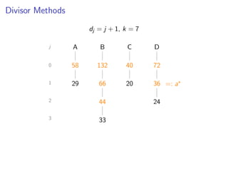
A = ai,j =
dj
vi
i ∈ [1..n], j ∈ N0
and obtain a = A(k) “directly”.](https://image.slidesharecdn.com/slides-160111170258/85/Practical-and-Worst-Case-Efficient-Apportionment-21-320.jpg)
![Reduction to Rank Selection
Observations
Knowing the value a selected last is sufficient.
We select the kth smallest value last.
Idea
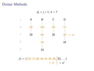
Use a selection algorithm on a finite subset of multiset
A = ai,j =
dj
vi
i ∈ [1..n], j ∈ N0
and obtain a = A(k) “directly”.](https://image.slidesharecdn.com/slides-160111170258/85/Practical-and-Worst-Case-Efficient-Apportionment-22-320.jpg)
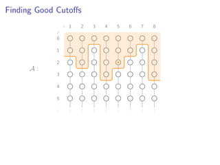
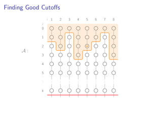
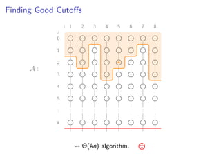
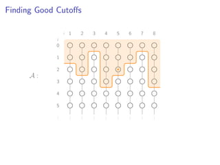
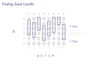
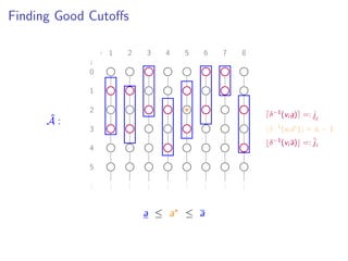
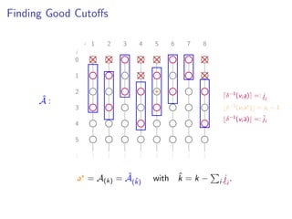
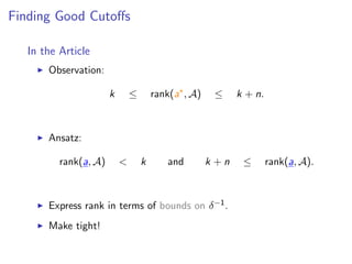
![Finding Good Cutoffs
Given (dj )j≥−1 with [technical details], we assume δ : R≥0 → R≥d0
with [technical details] so that
ai,j =
δ(j)
vi
and
δ−1
(y) = max{j ∈ Z≥−1 | dj ≤ y}
is the (zero-based) rank function of d.](https://image.slidesharecdn.com/slides-160111170258/85/Practical-and-Worst-Case-Efficient-Apportionment-27-320.jpg)
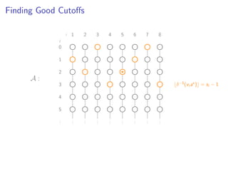
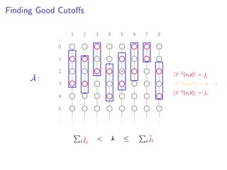
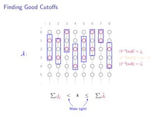
![Finding Good Cutoffs
i
j
1 2 3 4 5 6 7 8
0
1
2
3
4
5
...
...
...
...
...
...
...
...
...
[
[
[
[
[
]
]
]
]
]
]
]
]
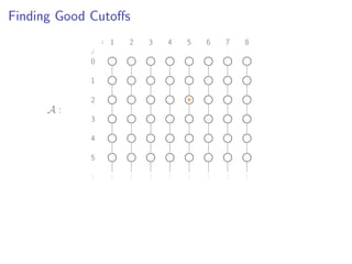
A :
δ−1(vi a ) = si − 1
δ−1(vi a)
δ−1(vi a)
a ≤ a ≤ a](https://image.slidesharecdn.com/slides-160111170258/85/Practical-and-Worst-Case-Efficient-Apportionment-30-320.jpg)
![Good Bounds On a
If
αx + β ≤ δ(x) ≤ αx + β
with β ≤ α and [technical details], then
a := max 0,
αk − (α − β) · n)
n
i=1 vi
and
a :=
αk + βn
n
i=1 vi
work.](https://image.slidesharecdn.com/slides-160111170258/85/Practical-and-Worst-Case-Efficient-Apportionment-37-320.jpg)
![Good Bounds On a
If
αx + β ≤ δ(x) ≤ αx + β
with β ≤ α and [technical details], then
a := max 0,
αk − (α − β) · n)
n
i=1 vi
and
a :=
αk + βn
n
i=1 vi
work.
Furthermore,
| ˆA| ≤ 2(1 + (β − β)/α) · n ∈ Θ(n) .](https://image.slidesharecdn.com/slides-160111170258/85/Practical-and-Worst-Case-Efficient-Apportionment-38-320.jpg)

![The Algorithm
RW15d (v, k) :
1. Compute a and a.
2. Initialize ˆA := ∅ and ˆk := k.
3. For each i ∈ [1..n] do:
3.1 Compute ji
and ji .
3.2 Add all dj/vi to ˆA for which ji
≤ j ≤ ji .
3.3 Update ˆk ← ˆk − ji
.
4. Select and return ˆA(ˆk).](https://image.slidesharecdn.com/slides-160111170258/85/Practical-and-Worst-Case-Efficient-Apportionment-41-320.jpg)
![The Algorithm
RW15d (v, k) :
1. Compute a and a.
2. Initialize ˆA := ∅ and ˆk := k.
3. For each i ∈ [1..n] do:
3.1 Compute ji
and ji .
3.2 Add all dj/vi to ˆA for which ji
≤ j ≤ ji .
3.3 Update ˆk ← ˆk − ji
.
4. Select and return ˆA(ˆk).
Θ
(n)
runtim
e!](https://image.slidesharecdn.com/slides-160111170258/85/Practical-and-Worst-Case-Efficient-Apportionment-42-320.jpg)
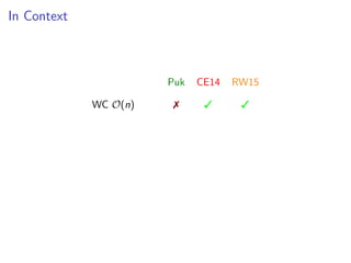
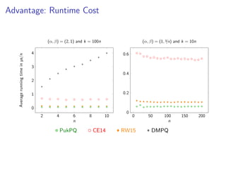
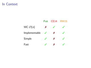
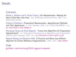

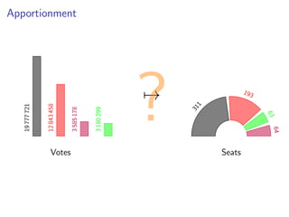
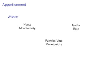
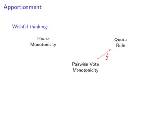
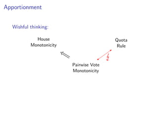
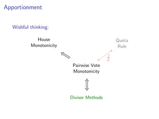
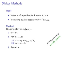
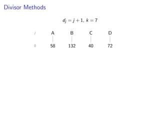
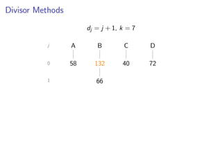
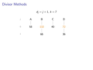
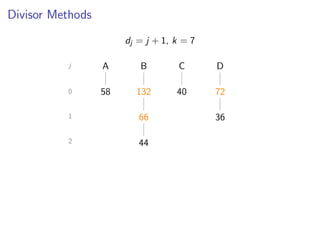
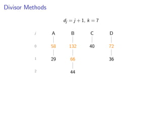
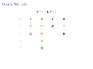
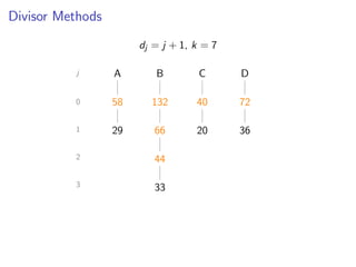
The document discusses practical and worst-case efficient apportionment algorithms developed by Raphael Reitzig and Sebastian Wild, focusing on divisor methods for allocating seats based on votes from multiple parties. It outlines various apportionment wishes like pairwise vote monotonicity and house monotonicity, as well as details computational methods for implementing these algorithms. Additionally, it includes runtime analysis and references to related literature on the topic.


![Arthur Vinnitsky Poster 4 [Autosaved]](https://cdn.slidesharecdn.com/ss_thumbnails/b5331afd-ff50-41f9-be04-4f662036c34c-160111170345-thumbnail.jpg?width=640&height=640&fit=bounds)


![谷歌留痕技术 [ 𝙩𝙤𝙥 𝟮𝟯𝟯. 𝙘 𝙤𝙢 ]](https://cdn.slidesharecdn.com/ss_thumbnails/top233-260130174328-3833018c-thumbnail.jpg?width=640&height=640&fit=bounds)


