This document is a master's thesis submitted by R.Q. Vlasveld to Utrecht University in partial fulfillment of the requirements for a Master of Science degree. The thesis explores using one-class support vector machines (SVMs) for temporal segmentation of human activity time series data recorded by inertial sensors in smartphones. The author first reviews related work in temporal segmentation and change detection methods. An algorithm is then presented that uses an incremental SVDD model to detect changes between activities in a continuous data stream. The algorithm is tested on both artificial and real-world human activity data sets recorded by the author. Quantitative and qualitative results demonstrate the method can find changes between activities in an unknown environment.


![Acronyms
ACRAS Almende Continuous Real-world Activities with on-body smartphones Sensors
Data Set. 4, 5, 52, 62, 64
AIC Akaike Information Criterion. 11
AR Autoregressive. 35, 40, 44
BIC Bayesian Information Criterion. 11
changeFinder is a unifying framework proposed by Takeuchi and Yamanishi [62] which
combines outlier detection and change detection. 16, 33
CUSUM Cumulative Sum. 7, 9–12, 34, 40, 41
FAR False Alarm Rate. 45–47, 53, 54, 65
GMM Gaussian Mixture Model. 19
HAR Human Activity Recognition. 1–5, 9, 14, 32, 60, 64
HMM Hidden Markov Model. 11
ICSS Iterated Cumulative Sums of Squares. 12
i.i.d. independently and identically distributed. 17
I-SVDD Incremental Support Vector Data Description. 34, 36–39, 61
KKT Karush-Kuhn-Tucker. 37
KL Kullback-Leibler. 17, 18
KLIEP Kullback-Leibler Importance Estimation Procedure. 10, 13
MLE Maximum Likelihood Estimates. 12
viii](https://image.slidesharecdn.com/593e322b-ac24-4819-ab2f-7f19350bcfbc-160327175441/85/thesis-9-320.jpg)
![Chapter 1
Introduction
With the wide availability of smartphones and built-in inertial sensors, more and more
applications of Human Activity Recognition (HAR) are introduced [6, 20, 27]. Many
approaches to recognize the performed activity rely on classification of recorded data
[5, 7, 11, 21, 33, 74, 77], which can be done online or in batches after the performance
[22]. Often time windows are used, which form short consecutive segments of data and
are processed in a model construction and recognition phase. The constructed model
is used to determine which (earlier learned) activity is performed. Besides the explicit
classification of the data, an implicit obtained result is a segmentation of performed
activities over time.
The goal of this thesis is to create an method for online temporal segmentation of time
series data. This will be performed explicitly, prior to the classification of data segments
to learned activities.
Our assumption is that a temporal segmentation of time series can be beneficial in-
formation for classification methods. Instead of using a fixed window approach, the
classification methods can use a larger set of homogeneous data. Thereby, the methods
have more information to create a solid model of the activities.
To find a temporal segmentation, we rely on change detection in time series. In the
context of this research the time series consists of recordings from inertial sensors dur-
ing the performance of human activities. The sensors, such as the accelerometer, are
nowadays widely available in smartphones. We are interested in real-world data from
both in- and outdoor activities performed in a continuous manner.
Compared to recordings in a controlled laboratory environment, we expect the real-
world data to be prone to unexpected characteristics. The constructed method must be
robust in order to handle these.
1](https://image.slidesharecdn.com/593e322b-ac24-4819-ab2f-7f19350bcfbc-160327175441/85/thesis-11-320.jpg)
![Chapter 1. Introduction 2
For the change detection algorithm we will use a special form of a SVM, the One-Class
Classification (OCC) based Support Vector Data Description (SVDD), as introduced by
Tax [63]. This method models the data in the shape of a high-dimensional hypersphere.
From this hypersphere the radius is extracted, which can be used as an indication of
change and be processed by one-dimensional change detection algorithms. The radius of
the hypersphere is used in the following relation. When the performed activity changes,
so will the data distribution and characteristics. This results in a change of the con-
structed model, especially in the radius of the hypersphere. Thus, a change in the radius
indicates a changes in the performed activity.
The remainder of this introduction is organized as follows. In Section 1.1 the scope of
this thesis is discussed. A short discussing on the workings of an One-Class Support
Vector Machine is provided in Section 1.2. The data sets we have used in this work are
discussed in Section 1.3. Section 1.4 gives a short overview of our contributions. Finally,
Section 1.5 outlines the structure of this thesis.
1.1 Scope
The scope of this thesis are segmentation methods of inertial sensor data in the field
of machine learning. The type of data is inertial sensor time series, collected by on-
body worn sensors as found in smartphones. These time series are recorded during the
performance of real-world human activities. The setting of the activities are real-world
environments, both in- and outdoor.
As mentioned in the previous section, a segmentation is often obtained as a by-product
from direct windowed classification. Other approaches have a very rigid form of segmen-
tation, e.g. by limiting the number of possible segment types [14, 35], or have applied
it to different type of time series data. In Fuchs et al. [24] artificial sinusoidal data is
processed. Li and Zheng [44] use visual motion data streams to find patterns of activ-
ities. The method of Guenterberg et al. [28] is able to distinguish periods of rest and
activity in inertial sensor data streams. Others have extracted features from windows of
data which are used for the segmentation [29]. These activities include sitting, standing,
walking, running, and ascending and descending staircases.
The problem of finding a temporal segmentation can be seen as a sub-problem to the
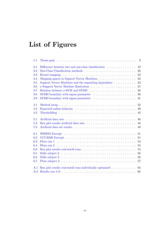
problem of Activity Classification. This relation is illustrated in Figure 1.1. The figure
visualizes that we can apply classification on time series data. In many approaches
it is applied to (partially overlapping) windows of data. In the context of HAR, the
window length commonly consists of around two seconds of data. In our setup we](https://image.slidesharecdn.com/593e322b-ac24-4819-ab2f-7f19350bcfbc-160327175441/85/thesis-12-320.jpg)
![Chapter 1. Introduction 3
perform temporal segmentation, instead of using a fixed window length. Each segment
will consist of homogeneous data, in the sense that the underlying data generating
activity should not change within a segment. Likewise, the previous and next segments
(if present) should be generated by a different activity.
Temporal Classification
Time series
Data
Activity
Classification
Temporal Segmentation
Model construction
Change detection
OC-SVM
model
Hypersphere
Radius
Classification
over windows
Figure 1.1: The goal of this thesis. The scope of this thesis is Temporal Segmentation,
which can be useful in the context of Temporal Classification. Given a data set, we
construct a OC-SVM high-dimensional spherical model, from which we extract the
radius. This metric is then applied to direct change detection algorithms. The detected
change points can support the classification of homogeneous segments of data.
To find these segments of homogeneous data, we employ a model construction phase.
The One-Class Support Vector Machine transforms the data to a higher dimensional
space. Non-linear mapping functions are used to add flexibility to the classification
decision boundary. In the higher dimensional space an enclosing boundary around the
data points, in the shape of a hypersphere, is constructed. The size, expressed as the
radius, of the hypersphere depends on the distribution of the data points in the model.
We will use the radius of this hypersphere as a characterizing metric and base our change
detection on it.
The model processes the data in windows of fixed length. A change in data distribution
and characteristics should then result in a change of the hypersphere’s radius. Such a
(sudden) change in the radius thus reflects a change in the time series data. It indicates
the end of the current and the beginning of a new segment. In Section 2.2 a detailed
overview of temporal segmentation methods is given. Information about segments can
be used in the classification phase of HAR. Instead of using relatively small windows, it
can apply classification to the full segments of data. The final result, which is outside
the scope is this thesis, will be a full classification of activities over the time series data.
1.2 One-Class Support Vector Machines
In the setup, as described in the previous section and visualized in Figure 1.1, we employ
a model construction phase. For this model we will use an One-Class Support Vector
Machine implementation: the Support Vector Data Description algorithm by Tax [63].
In earlier research multi-class SVMs are used for direct classification of inertial sensor](https://image.slidesharecdn.com/593e322b-ac24-4819-ab2f-7f19350bcfbc-160327175441/85/thesis-13-320.jpg)
![Chapter 1. Introduction 4
data [5, 33, 51]. Others have used OC-SVM classifiers for novelty or outlier detection
[13, 45, 48, 58, 64]. The method by Yin et al. [78] creates a OC-SVM classifier to filter
normal activity traces, using training data. However, to the best of our knowledge,
OC-SVM methods have not yet been applied to inertial sensor time series data directly
to find changes in behavior and create a temporal segmentation.
The OC-SVMs algorithms transforms the time series data, which can be of any high
dimension, to a higher dimensional feature space. When the data is assumed to be of
the same class, it can be characterized by an enclosing boundary. In case of the SVDD
algorithm this boundary is in the shape of a hypersphere. Using this model, we are able
to test the membership of a new data point to the described class. The new data point
is transformed to the feature space and its location is compared to the boundary. If it
lies within the boundary then it is a member of the class and otherwise it is regarded as
an outlier.
In case the data distribution changes, the data points will have a larger variance. It
will result in a larger hypersphere in the feature space. This means that a change
in the underlying process of a time series data results in a larger hypersphere radius.
Thus the OC-SVM method allows us to reduce a complex high-dimensional signal to an
one-dimensional time series data. The reduced time series can be inspected by simpler
change detection methods, in a number of ways. Chapter 3 will discuss the OC-SVM
methods in detail and Chapter 4 elaborates on the overall change detection method.
1.3 Data sets
In recent research two data sets for HAR have been made public. In order to benchmark
our proposed method we applied our method to these data sets. However, it turned out
the data sets were not appropriate for continuous temporal segmentation. In the Wire-
less Sensor Data Mining (WISDM) set [43] the activities are not performed continuously.
There is no transition period between activities. Since we are interested in the detection
changes between consecutive activities, we can not use this data set. The Human Activ-
ity Recognition Using Smartphones Data Set (UCI HAR) from [5] also lacks continuous
recordings. Furthermore, it seems to have incorrect labels. Finally, for both data sets
there are no visual images of the performed activities. So in case of ambiguity there is
no ground truth to consult. To overcome these problems, we have created our own real-
world data set: Almende Continuous Real-world Activities with on-body smartphones
Sensors Data Set [72].](https://image.slidesharecdn.com/593e322b-ac24-4819-ab2f-7f19350bcfbc-160327175441/85/thesis-14-320.jpg)
![Chapter 1. Introduction 5
Our own data set is recorded by placing a smartphone with inertial sensors in the front
right pants pocket of a subject. The subject was asked to perform common and simple
activities in a natural environment, both in- and outdoors. During the performance the
subjects were also recorded with a video camera from a third-person point of view. This
allows us to create a ground truth for the temporal segmentation of performed activities.
Besides the recorded data sets we have used artificial data sets to obtain an objective,
quantitative, performance measure of the method. These artificial data sets are modeled
to the sets used in [13, 62]. In Chapter 5 we discuss the artificial data sets and results
in detail. The real-world recordings and results are discussed in Chapter 6.
1.4 Contributions
As a result from our proposed method and application to recorded real-world data sets,
this thesis will provide the following contributions:
1. Continuous recorded human activity data: the proposed method is applied
to our own recorded human activity data. This data set can be grounded by
using the video recordings of the subject while performing the activities. The data
set, consisting of raw inertial sensor recordings, manual change point and activity
labeling, and video recordings, is used for testing the method and is made available
to the public [72].
2. Application of OC-SVM methods to inertial sensor data: to the best of our
knowledge, this thesis is the first application of OC-SVM methods, especially the
SVDD method, to inertial sensor signals in the context of temporal segmentation.
Furthermore, this thesis contributes to research that has temporal segmentation
of inertial sensor data as its primary objective.
3. Adaptation of SVCPD: we have adopted and simplified the SVCPD method by
Camci [13] in order to find change points in time series data. In our simplification
we have not encountered a noticeably decrease in performance.
1.5 Thesis structure
The structure of this thesis is as follows. In Chapter 2 a literature review is provided.
We will look at the different interpretations and implementations for change, novelty,
and outlier detection. Previous work in the field of HAR is discussed and we end with](https://image.slidesharecdn.com/593e322b-ac24-4819-ab2f-7f19350bcfbc-160327175441/85/thesis-15-320.jpg)
![Chapter 1. Introduction 6
existing applications of SVMs to change detection. Chapter 3 further analyses SVMs
and two implementations of OC-SVMs. It relates the properties of the constructed OC-
SVM models to change detection in time series data. That relation is applied to our
problem formulation in Chapter 4, where we construct our change detection method
One-Class SVM Human Activity Temporal Segmentation (OCS-HATS) [73], based on
the work of Camci [13]. In Chapter 5 we apply the method to artificial data and show
the quantitative performance. In Chapter 6 the method is applied to our real-world
Almende Continuous Real-world Activities with on-body smartphones Sensors Data Set
(ACRAS) [72]. In that chapter we show, by qualitative analysis, the ability of detecting
change in HAR data, recorded by inertial sensors. This thesis is concluded in Chapter 7,
in which we reflect on the performed research and state possibilities for feature research.](https://image.slidesharecdn.com/593e322b-ac24-4819-ab2f-7f19350bcfbc-160327175441/85/thesis-16-320.jpg)
![Chapter 2. Literature review 8
The widely used Cumulative Sum (CUSUM) method by Basseville et al. [10] follows
this approach. It originates from quality control and benchmarking methods for manu-
facturing processes. This method, and some derivatives, are discussed and analyzed in
Section 2.2.2.
Many methods rely on pre-specified parametric model assumptions and consider the
data to be independent over time, which makes it less flexible to real-world applications.
The methods proposed by Kawahara et al. [40] and Lui et al. [46] try to overcome
these problems by estimating the ratio between the PDFs of time windows, instead of
estimating each PDF. This approach is discussed and analyzed in Section 2.3.
The density-estimation methods rely on the log-likelihood ratio between PDFs. The
method of Camci [13] follows an other approach within the statistical framework, by
using an SVM. One problem it tries to overcome is the (claimed) weakness of many
methods to detect a decrease in variance. The method represents the distribution over
the data points as a hypersphere in a higher dimension. A change in the PDF is repre-
sented by a change in the radius of this sphere. In Section 2.4 more applications of the
SVM-based methods are discussed. Since OCC and the OC-SVM method is central in
our approach, Sections 3.2 and 3.3 discuss these techniques in detail.
In the search for the change in properties, temporal segmentation and change point
detection methods can roughly be categorized in four methods in the way the data is
processed, as discussed by Avci et al. [6]:
1. Top-Down methods iteratively divide the signal in segments by splitting at the
most optimal location. The algorithm starts with two segments and completes
when a certain condition is met, such as when an error value or number of segments
k is reached.
2. Bottom-Up methods are the natural complement to top-down methods. They
start with creating n/2 segments and iteratively join adjacent segments while the
value of a cost function for that operation is below a certain value.
3. Sliding Window methods are simple and intuitive for online segmentation. It
starts with a small initial subsequence of the time series. New data points are
added to the current segment until the fit-error is above a threshold.
4. Sliding Window And Bottom-up, as introduced by Keogh et al. [41], combines
the ability of the sliding window mechanism to process time series online and
the bottom-up approach to create superior segments in terms of fit-error. The
algorithm processes the data in two stages. The first stage is to join new data
points in the current segment created by a sliding window. The second stage](https://image.slidesharecdn.com/593e322b-ac24-4819-ab2f-7f19350bcfbc-160327175441/85/thesis-18-320.jpg)
![Chapter 2. Literature review 9
processes the data using Bottom-Up and returns the first segment as the final
result. Since this second stage retains some (semi-)global view of the data, the
results are comparative with normal Bottom-Up while being able to process the
data in an online manner.
For the application of this research Sliding Window and preferably Sliding Window
And Bottom-up (SWAB)-based algorithms will be considered. In the following sections
we discuss classes of algorithms grouped by the type of decision function, assuming a
SWAB-based data processing order.
2.2 Temporal Segmentation
This section gives an overview of the literature on temporal segmentation in the context
of HAR. It provides a look on different implementations and methodologies. A wide
range of terms and subtle differences are used in the field, such as ‘segmentation’, ‘change
detection’, ‘novelty detection’ and ‘outlier detection’. The following sections discuss
these different methods.
2.2.1 Segmentation methods overview
Methods that apply temporal segmentation on time series data can be roughly cate-
gorized in three different methods, as discussed by Avci et al. [6]. In that survey the
distinction between Top-Down, Bottom-Up, and Sliding-Window approaches is based on
the way data is processed by the algorithm. Since we are interested in on-line change
detection, the literature discussed in this section will mainly be forms of sliding-window
algorithms.
In Keogh et al. [41] a comparison of the aforementioned approaches is made. The research
also introduces the SWAB method, which combines the simple and intuitive approach of
the sliding-window approach with the (semi-)global view over the data from the bottom-
up method. Each segment is approximated by a Piecewise Linear Representation (PLR),
within a certain error. The user-provided error threshold controls the granularity and
number of segments.
Other methods have been proposed, such as an adaptive threshold based on the signal
energy by Guenterberg et al. [28], the adaptive CUSUM-based test by Alippi et al. [3]
and the Moving Sum (MOSUM) by Hsu [37] in order to eliminate this user dependency.
The latter of these methods is able to process the accelerometer values directly, although](https://image.slidesharecdn.com/593e322b-ac24-4819-ab2f-7f19350bcfbc-160327175441/85/thesis-19-320.jpg)
![Chapter 2. Literature review 10
better results are obtained when features of the signal are processed, as done in the first
method [28]. Here the signal energy, mean and standard deviation are used to segment
activities and by adding all the axial time series together, the Signal-To-Noise ratio is
increased, resulting in a robuster method.
The method of Guenterberg et al. [28] extracts features from the raw sensor signal to base
the segmentation on other properties than the pure values. The method of Bernecker et
al. [11] uses other statistical properties, namely autocorrelation, to distinguish periodic
from non-periodic segments. Using the SWAB method the self-similarity of a one-
dimensional signal is obtained. The authors claim that only a slight modification is
needed to perform the method on multi-dimensional data. After the segmentation phase,
the method of Bernecker et al. [11] extracts other statistical features which are used in
the classification phase.
The proposal of Guo et al. [29] dynamically determines which features should be used for
the segmentation and simultaneously determines the best model to fit the segment. For
each of the three dimensions features such as the mean, variance, covariance, correlation,
energy and entropy are calculated. By extending the SWAB method, for every frame
a feature set is selected, using an enhanced version of Principal Component Analysis
(PCA). The research also considered the (Stepwise) Feasable Space Window as intro-
duced by [47], but since it results in a higher error rate than SWAB, the latter was
chosen to extend. Whereas the above mentioned algorithms use a linear representation,
this methods considers linear, quadratic and cubical representations for each segment.
This differs from other methods where the model is fixed for the whole time series, such
as [24], which is stated to perform inferior on non-stationary time series, such as those
from daily life.
The time series data from a sensor can be considered as being drawn from a certain
stochastic process. The CUSUM-methods instead follows a statistical approach and re-
lies on the log-likelihood ratio [31] to measure the difference between two distributions.
To calculate the ratio, the probability density functions need to be calculated. The
method of Kawahara et al. [40] proposes to estimate the ratio of probability densities
(known as the importance), based on the log likelihood of test samples, directly, without
explicit estimation of the densities. The method by Liu et al. [46] uses a compara-
ble dissimilarity measure using the Kullback-Leibler Importance Estimation Procedure
(KLIEP) algorithm. They claim this results in a robuster method for real-world scenar-
ios. Although this is a model-based method, no strong assumptions (parameter settings)
are made about the models.
The method of Adams and MacKay [56] builds a probabilistic model on the segment
run length, given the observed data so far. Instead of modeling the values of the data](https://image.slidesharecdn.com/593e322b-ac24-4819-ab2f-7f19350bcfbc-160327175441/85/thesis-20-320.jpg)
![Chapter 2. Literature review 11
points, the length of segments as a function of time is modeled by calculating its posterior
probability. It uses a prior estimate for the run length and a predictive distribution for
newly-observed data, given the data since the last change point. This method differs
from the approach of Guralnik and Srivastava [30] in which change points are detected by
a change in the (parameters of an) fitted model. For each new data point, the likelihoods
of being a change point and part of the current segment are calculated, without a prior
model (and thus this is a non-Bayesian approach). It is observed that when no change
point is detected for a long period of time, the computational complexity increases
significantly.
Another application of PCA is to characterize the data by determining the dimensional-
ity of a sequence of data points. The proposed method of Berbiˇc et al. [8] determines the
number of dimensions (features) needed to approximate a sequence within a specified
error. With the observation that more dimensions are needed to keep the error below
the threshold when transitions between actions occur, cut-points can be located and
segments will be created. The superior extension of their approach uses a Probabilistic
PCA algorithm to model the data from dimensions outside the selected set with noise.
In the method by Himberg et al. [35] a cost function is defined over segments of data.
By minimizing the cost function it creates internally homogeneous segments of data.
A segment reflects a state in which the devices, and eventually its user, are. The cost
function can be any arbitrary function and in the implementation the sum of variances
over the segments is used. Both in a local and global iterative replacement procedure (as
an alternative for the computationally hard dynamic programming algorithm) the best
breakpoint locations ci for a pre-defined number of segments 1 ≤ i ≤ k are optimized.
As stated before, often methods obtain an implicit segmentation as a result of clas-
sification over a sliding window. The method of Yang et al. [76] explicitly performs
segmentation and classification simultaneously. It argues that the classification of a pre-
segmented test-sequences becomes straightforward with many classical algorithms to
choose from. The algorithm matches test examples with the sparsest linear representa-
tion of mixture subspace models of training examples, searching over different temporal
resolutions.
The method of Chamroukhi et al. [14] is based on a Hidden Markov Model (HMM) and
logistic regression. It assumes a K-state hidden process with a (hidden) state sequence,
each state providing the parameters (amongst which the order) for a polynomial. The
order of the model segment is determined by model selecting, often using the Bayesian
Information Criterion (BIC) or the similar Akaike Information Criterion (AIC) [2], as
in [33].](https://image.slidesharecdn.com/593e322b-ac24-4819-ab2f-7f19350bcfbc-160327175441/85/thesis-21-320.jpg)
![Chapter 2. Literature review 12
2.2.2 CUSUM
An other often used approach in the statistical framework of change detection is the
CUSUM as introduced by Page [54]. Originally used for quality control in production
environments, its main function is to detect change in the mean of measurements [10].
It is a non-Bayesian method and thus has not explicit prior belief for the change points.
Many extensions to this method have been proposed. Some focus on the change in
mean, such the method of Alippi and Roveri [3]. Others apply the method the problems
in which the change of variance is under consideration. Among others are there the
centered version of the cumulative sums, introduced by Brown, Durbin and Evans [12]
and the MOSUM of squares by [37].
The method of Incl´an and Tiao [38] builds on the centered version of CUSUM [12]
to detect changes in variance. The obtained results (when applied to stock data) are
comparable with the application of Maximum Likelihood Estimates (MLE). Using the
batch Iterated Cumulative Sums of Squares (ICSS) algorithm they are able to find
multiple change points, offline while post-processing the data. Whereas CUSUM can be
applied to search for a change in mean, the ICSS is adapted to find changes in variance.
Let Ck = k
i=1 α2
t be the cumulative sum of squares for a series of uncorrelated random
variables {αt} of length T. The centered (and normalized) sum of squares is defined as
Dk =
Ck
CT
−
k
T
, k = 1, . . . , T, with D0 = DT = 0. (2.1)
For a series with homogeneous variance, the value of Dk will oscillate around 0. This
Dk is used to obtain a likelihood ratio for testing the hypothesis of one change against
no change in the variance. In case of a sudden change, the value will increase and
exceed some predefined boundary with high probability. By using an iterative algorithm,
the method is able to minimize the masking effect of successive change points. The
proposal of [17] extends on the CUSUM-based methods to find change points in mean
and variance, by creating a more efficient and accurate algorithm.
One of the motivations for the ICSS algorithm was the heavy computational burden
involved with Bayesian methods, which need to calculate the posterior odds for the log-
likelihood ratio testing. The ICSS algorithm avoids applying a function at all possible
locations, due to the iterative search. The authors recommend the algorithm for analysis
of long sequences.](https://image.slidesharecdn.com/593e322b-ac24-4819-ab2f-7f19350bcfbc-160327175441/85/thesis-22-320.jpg)
![Chapter 2. Literature review 13
2.2.3 Novelty and Outlier detection
In the case of time series data, many approaches rely on the detection of outlier, or
novel, data objects. An increase in outlier data objects indicates a higher probability of
change, as discussed by Takeuchi and Yamanischi [62]. The concepts of novelty detection
and outlier detection are closely related and often used interchangeable.
The algorithm by Ma and Perkins [49] uses Support Vector Regression (SVC) to model
a series of past observations. Using the regression, a matching function V (t0) is con-
structed which uses the residual value of t0 to create an outlier (out-of-class) confidence
value. The method defines novel events as a series of observations for which the outlier
confidence is high enough. In an alternative approach by the same authors [48] a classi-
fication method, in contrast with regression, is used to detect outlier observations. The
latter approach uses the ν-Support Vector Machine (ν-SVM) algorithm by Sch¨olkopf et
al. [58], which is further discussed in Section 2.4
A extensive overview of novelty detection based on statistical models is given by Markou
and Singh [49]. In the second part of their review [50], novelty detection by a variety
of neural networks is discussed. The survey by Hodge and Austin [36] distinguishes
between three types of outlier detection: 1) unsupervised, 2) supervised, and 3) semi-
supervised learning. As we will see in Section 3.2, in this research we are interested in
methods from Type 3, of which OCC is a member. More theoretical background on
outliers in statistical data is provided in the work by Barnett and Lewis [9].
2.3 Change-detection by Density-Ratio Estimation
Many approaches to detect change points monitor the logarithm of the likelihood ratio
between two consecutive intervals. A change point is regarded to be the moment in time
when the underlying probabilistic generation function changes. Some methods which
rely on this are novelty detection, maximum-likelihood estimation and online learning
of autoregressive models [40]. A limitation of these methods is that they rely on pre-
specified parametric models. Non-parametric models, for which the number and nature
of the parameters are undetermined, for density estimation have been proposed, but
it is said to be a hard problem [32, 61]. A solution to this is to estimate the ratio
of probabilities instead of the probabilities themselves. One of the recent methods to
achieve this is the KLIEP by Sugiyama et al. [60].
The proposed method by Kawahara and Sugiyama [40] uses an online version of the
KLIEP algorithm. It considers sequences of samples (rather than samples directly)](https://image.slidesharecdn.com/593e322b-ac24-4819-ab2f-7f19350bcfbc-160327175441/85/thesis-23-320.jpg)
![Chapter 2. Literature review 14
because the time series samples are generally not independent over time. The method
detects change by monitoring the logarithm of the likelihood ratio between densities of
reference (past) and test (current) time intervals. If it exceeds a predetermined threshold
value, the beginning of the test interval is marked as a change point.
Since the density ratio is unknown, it needs to be estimated. The naive approach is
to estimate it using estimated densities of the two intervals. Since this is known to be
a hard problem and sensitive for errors, the solution would be to estimate the ratio
directly.
The method by Liu et al. [46] estimates the ratio of probabilities directly, instead of
estimating the densities explicitly. Other methods using ratio-estimation are the Un-
constrained Least-Squares Importance Fitting (uLSIF) method [39], and an extension
which possesses a superior non-parametric convergence property: Relative uLSIF (RuL-
SIF) [75].
2.4 Support Vector Machines in Change Detection
Many proposals in the field of HAR make use of SVMs as a (supervised) model learning
method. An elaborate overview of applications is given in [51]. In this section we review
methods of change detection based on the applications of SVMs as model construction
method. Sch¨olkopf et al. [58] applies Vapnik’s principle never to solve a problem which
is more general than the one that one is actually interested in. In the case of novelty
detection, they argue there is no need for a full density estimation of the distribution.
Some algorithms estimate the density by considering how many data points fall in a
region of interest. The ν-SVM method instead starts with the number of data points
that should be within the region and estimates a region with that desired property. It
builds on the method of Vapnik and Vladimir [70], which characterizes a set of data
points by separating it from the origin. The ν-SVM method adds the kernel method,
allowing non-linear decision functions, and incorporates ‘softness’ by the ν-parameter.
Whereas the method in [70] focuses on two-class problems, the ν-SVM method solves
one-class problems.
The method introduced by Ma and Perkins [48] creates a projected phase of a time series
data, which is intuitively equal to applying a high-pass filter to the time series. The
projected phase of the time series combines a history of data points to a vector, which
are then classified by the ν-SVM method. The method is applied to a simple synthetic
sinusoidal signal with small additional noise and a small segment with large additional
noise. The algorithm is able to detect that segment, without false alarms.](https://image.slidesharecdn.com/593e322b-ac24-4819-ab2f-7f19350bcfbc-160327175441/85/thesis-24-320.jpg)
![Chapter 2. Literature review 15
The algorithms of SVMs has been applied to the problem of HAR, as by Anguita et al.
[5]. In that research a multi-class classification problem is solved using SVMs and the
One-Vs-All method. The method exploits fixed-point arithmetic to create a hardware-
friendly algorithm, which can be executed on a smartphone.1
With the same concepts as ν-SVM, the SVDD method by Tax and Duin [64, 65] uses
a separating hypersphere (in contrast with a hyperplane) to characterize the data. The
data points that lie outside of the created hypersphere are considered to be outliers,
which number is a pre-determined fraction of the total number of data points.
The method by Yin et al. [78] uses the SVDD method in the first phase of a two-
phase algorithm to filter commonly available normal activities. The Support Vector
based Change Point Detection (SVCPD) method of Camci [13] uses SVDD applies it to
time-series data. By using an OC-SVM the method is able to detect changes in mean
and variance. Especially the detection of variance decrease is an improvement over other
methods that are unable to detect decreases in variance [62]. This main research subject
of this thesis is to apply the method of Camci [13] to sensor data (such as accelerometer
time series) obtained by on-body smartphones.
The following chapter discusses OCC, OC-SVM, and change detection through OC-SVM
in detail. It will show that the used implementation of OC-SVM is an example of the
Type 3 semi-supervised learning methods, in the system of Hodge and Austin [36].
1
Smartphones have limited resources and thus require energy-efficient algorithms. Anguita et al. [4]
introduce a Hardware-Friendly SVM. It uses less memory, processor time, and power consumption, with
a loss of precision.](https://image.slidesharecdn.com/593e322b-ac24-4819-ab2f-7f19350bcfbc-160327175441/85/thesis-25-320.jpg)
![Chapter 3
Change detection by Support
Vector Machines
This chapter discusses the concepts and algorithms that will be used as a basis for the
proposed method, as introduced in Chapter 4. The first section formulates the problem
of change detection and relates it to outlier and novelty detection. It transforms the
traditional problem of outlier detection into change detection for times series data. In
Section 3.2 the problem of One-Class Classification is explained and discusses a number
of implementations. In the final sections of this chapter, Section 3.3, two SVM-based
OCC methods, ν-SVM and SVDD, and the influence of model parameters are further
discussed in detail.
3.1 Problem Formulation of Change Detection
The problems of outlier and novelty detection, segmentation, and change detection in
time series data are closely related. The terminology depends on the field of application,
but there are subtle differences. The problem of outlier detection is concerned with
finding data objects in a data set which have small resemblance with the majority of
the data objects. These objects can be regarded as erroneous measurements. In the
case of novelty detection these objects are considered to be member of a new class of
objects. The unifying framework of Takeuchi and Yamanishi [62], changeFinder, creates
a two stage process expressing change detection in terms of outlier detection. The first
stage determines the outliers in a time series by giving a score based on the deviation
from a learned model, and thereby creates a new time series. The second stage runs
on that new created time series and calculates a average over a window of the outlier
scores. The problem of change detection is then reduced to outlier detection over that
16](https://image.slidesharecdn.com/593e322b-ac24-4819-ab2f-7f19350bcfbc-160327175441/85/thesis-26-320.jpg)
![Chapter 3. Change detection by Support Vector Machines 17
average-scored time series. The implementation by Camci [13], SVCPD, implements
outlier detection with the SVDD algorithm to detect changes in mean and variance.
The problem of change point detection can be formulated using different type of models,
as discussed in 2.2.1. The methods by Takeuchi and Yamanishi [62] and Camci [13] use
the following formulation for change detection, which we will also use for our problem
formulation. The algorithm searches for sudden changes in the time series data. In other
words, slowly changing properties in the data are not considered to be changes. Consid-
ered a time series x1, x2, . . . , which is drawn from a stochastic process p. Each xt (t =
1, 2, . . . ) is a d-dimensional real valued vector. Assume p can be “decomposed” in two
different independently and identically distributed (i.i.d.) stationary one-dimensional
Gaussian processes p(1) and p(2). Consider a potential change point at time a. Data
points x1, . . . , xa−1 ∼ N(µ1, σ2
1) = p(1) and xa, . . . , xt ∼ N(µ2, σ2
2) = p(2). If p(1) and
p(2) are different (enough), then the time point t = a is marked as a change point.
Takeuchi and Yamanishi [62] expess the similarity between the stochastic processes with
the Kullback-Leibler (KL) divergence D(p2||p1). It is observed that their method is not
able to detect a change by decrease in variance [13, 62]. This problem is the motivation
for Camci [13] to create the SVCPD algorithm.
The definition of change point being sudden changes in the time series data is in line with
the search of changes in activities. Since we are only interested in different activities
(which are represented by sudden changes), slight changes within an activity are not of
interest.
3.2 One-Class Classification
As discussed in the previous section, change detection in time series can be implemented
using outlier, or novelty, detection. To regard a data point as an outlier, there must
be a model of the normal time series data and a (dis)similiarity measure defined over
the model and data objects. When a data point differs enough from the created model,
it can be labeled as an outlier. The class of OCC algorithms is especially designed for
that purpose. The algorithms build up a model of the data, assuming only normal data
objects are available (or a very limited amount of example outlier data objects). This
is also known as novelty detection or semi-supervised detection and is of Type 3 in the
system by Hodge and Austin [36]. This differs from classical classification algorithms,
which commonly rely of both positive and negative examples.](https://image.slidesharecdn.com/593e322b-ac24-4819-ab2f-7f19350bcfbc-160327175441/85/thesis-27-320.jpg)
![Chapter 3. Change detection by Support Vector Machines 18
In Section 3.2.1 the problem formulation of OCC methods is explained. In section 3.2.2
an overview of OCC methods is given. The following section will discuss one specific set
of methods, the OC-SVM which use SVMs to model the normal training data.
3.2.1 Problem formulation
The problem of One-Class Classification is closely related to the (traditional) two-class
classification situation1. In the case of traditional classification algorithms, the problem
is to assign an unknown object to one of the pre-defined categories. Every object i is
represented as a d-dimensional vector xi = (xi,1, . . . , xi,d), xi,j ∈ R. Using this notation,
an object xi thus represents one point in a feature space X ∈ Rd. The two classes
of objects, ω1 and ω2, are labeled −1 and +1 respectively. The objects with a label
yi ∈ {−1, +1} are in the training set (note that it can be both positive and negative
example objects). This problem is solved by determining a decision boundary in the
feature space of the data objects and label the new data object based on the location
relative to this boundary. This is expressed by the decision function y = f(x):
f : Rd
→ {−1, +1} (3.1)
In case of the OCC problem, only one class (often referred as the target class, or positive
examples) of training data is used to create a decision boundary. The goal is to determine
whether a new data object belongs to the target class. If it does not belong to the class
it is an outlier. One could argue that this problem is equal to the traditional two-
class problem by considering all other classes as negative examples, although there are
important differences. In pure OCC problems there are no negative example objects
available. This could be because the acquisition of these examples is very expensive, or
because there are only examples of the ‘normal’ state of the system and the goal is to
detect ‘abnormal’ states. Since the algorithm’s goal is to differentiate between normal
and abnormal objects (relative to the training objects), OCC is often called outlier,
novelty or anomaly detection, depending on the origin of the problem to which the
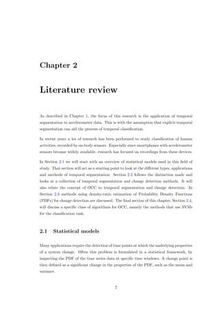
algorithm is applied2. The difference between two and one-class classification and the
consequence for outlier objects is illustrated in Figure 3.1. In the two-class classification
problem the object o will be member of the -1 class whilst the OCC problem will label
it as an outlier. In [63] a more detailed analysis of the OCC is given.
The OCC algorithms have been applied to a wide range of applications. The first is,
obviously, outlier detection of objects which do not resemble the bulk of the training
1
Two-class problems are considered the basic problem, since multi-class classification problems can
be decomposed into multiple two-class problems [25].
2
The term One-Class Classification originates from Moya et al. [52].](https://image.slidesharecdn.com/593e322b-ac24-4819-ab2f-7f19350bcfbc-160327175441/85/thesis-28-320.jpg)
![Chapter 3. Change detection by Support Vector Machines 19
x
y
+
+
+
+
+
+
+
+
+
+
+
+
-
+
++
+
+
+
+
o
- -
-
-
--
-
-
-
-
- -
-
-
--
-
-
-
-
-
-
-
-
-
--
-
Figure 3.1: This plot shows the difference between two and one-class classification.
The solid line indicates a possible decision boundary between the +1 and -1 example
objects. The dashed circle indicates the closed boundary around all the data objects.
In the first type the object o is considered to be member of the -1-class, whilst in the
latter (OCC) formulation it is an outlier.
data. It can be a goal by itself and can be used as a filtering mechanism for other data
processing methods. Often methods that rely on data characteristics are sensitive for
remote regions in the data set. Using OCC these remote regions can be removed from
the data set. A second application is for the problem as described above, in which only
data from a single target class is available. When this problems originates from e.g.
a monitoring process, the OCC is able to recognize abnormal system states, without
the need to create (or simulate) faulty states beforehand. The final possible application
given by Tax [63] is the comparison of two data sets. By constructing a OCC-classifier
using a training data set, one can compare that set to a new data set. This will result
in a similarity measure expressed in the properties of outliers. This is related to other
methods of expressing similarity, such as density-ratio estimation and the KL divergence
as discussed in Section 3.1.
3.2.2 One-Class Classification methods
The methods and algorithms used for the OCC-problem can be organized into three
categories [53, 63], visually represented in Figure 3.2. The first category consists of
methods that estimate the density of the training data and set a threshold on this den-
sity. Among those are Gaussian models, Gaussian Mixture Models (GMMs) and Parzen
density estimators. In order to get good generalization results with these methods, the
dimensionality of the data and the complexity of the density need to be restricted. This](https://image.slidesharecdn.com/593e322b-ac24-4819-ab2f-7f19350bcfbc-160327175441/85/thesis-29-320.jpg)
![Chapter 3. Change detection by Support Vector Machines 20
One-Class Classification
methods
Density Estimation Reconstruction
methods
Boundary methods
Gaussian Model
Gaussian
Mixture Model
Parzen density
estimation
K-means, LVQ,
SOM
PCA
Mixture of PCAs
K-centers
Nearest
neighborhood
Support Vector
Data Description
Neural networks...
...
...
Figure 3.2: Overview of OCC methods categorized in Density Estimation, Recon-
struction methods, and Boundary methods. This categorization follows the definition
of Tax in [63].
can cause a large bias on the data. When a good probability model is postulated, these
methods work very well.
Boundary methods are based on Vapnik’s principle3 which imply in this case that es-
timating the complete data density for a OCC may be too complex, if one is only
interested in the closed boundary. Examples of methods that focus on the boundary (a
direct threshold) of the training data distribution are K-centers, Nearest-neighborhood,
and SVDD, or a combination of those methods [34]. Especially SVDD has a strong bias
towards minimal volume solutions. These type of methods are sensitive to the scale and
range of features, since they rely on a well-defined distance measure. The number of
objects that is required, is smaller than in the case of density methods. The boundary
method SVDD, constructed by Tax and which has shown good performance [42], will
be further discussed in Section 3.3.4.
Reconstruction methods take a different approach. Instead of focusing on classification
of the data and thus on the discriminating features of data objects, they model the
data. This results in a compact representation of the target data and for any object a
reconstruction error can be defined. Outliers are data objects with a high error, since
they are not well reconstructed by the model. Examples of reconstruction methods are
K-means, PCA and different kind of neural network implementations.
In [42, 53] an overview of applications for OCC-algorithms, and explictly for SVM-
based methods (such as SVDD and ν-SVM), is given. It shows succesful applications
3
With a limited amount of data available, one should avoid solving a more general problem as an
intermediate step to solve the original problem [71].](https://image.slidesharecdn.com/593e322b-ac24-4819-ab2f-7f19350bcfbc-160327175441/85/thesis-30-320.jpg)
![Chapter 3. Change detection by Support Vector Machines 21
for, amonst others, problems in the field of Handwritten Digit Recognition, Face Recog-
nition Applications, Spam Detection and Anomaly Detection [45, 55]. As discussed in
Section 3.1, this can be used for change detection in time series data.
In this Section we have discussed the problem of OCC and different kind of implemen-
tations. An often used implementation is the SVM-based method [53], since is shows
good performance in comparitive researches [42, 59]. In the following section (3.3) two
implementations of OC-SVM will be discussed, the SVDD method of Tax and Duin [64]
and the ν-SVM-algoritm by Sch¨olkopf.
3.3 One-Class Support Vector Machine
In this section we will discuss the details of an SVM and OC-SVM implementations.
The classical implementation of an SVM is to classify a dataset in two distinct classes.
This is a common use case, although sometimes there is no training data for both classes
available. Still, one would like to classify new data points as regular, in-class, or out-
of-class, e.g. in the case of a novelty detection. With that problem only data examples
from one class are available and the objective is to recognize new data points that are
not part of that class. This unsupervised learning problem is closely related to density
estimation. In that context, the problem can be the following. Assume an underlying
probability distribution P and a data point x drawn from this distribution. The goal is
to find a subset S of the input space, such that the probability that x lies inside of S
equals some predetermined value ν between 0 and 1 [58].
In the following of this section we will start with a discussion of traditional SVMs. In
Section 3.3.2 we will show how kernels allow for non-linear decision functions. That
is followed by two different implementations of OC-SVM: ν-SVM in Section 3.3.3 by
Sch¨olkopf et al. [58], which closely follows the above problem statement regarding density
estimation, and SVDD by Tax and Duin [64] in Section 3.3.4. The final part of this
section discusses the influence of model parameters on the performance of SVMs
3.3.1 Support Vector Machine
We will first discuss the traditional two-class SVM before we consider the one-class
variant, as introduced by Cortes and Vapnik in [19]. Consider a labeled data set Ω =
{(x1, y1), (x2, y2), . . . , (xn, yn)}; points xi ∈ I in a (for instance two-dimensional) space
where xi is the i-th input data point and yi ∈ {−1, 1} is the i-th output value, indicating
the class membership.](https://image.slidesharecdn.com/593e322b-ac24-4819-ab2f-7f19350bcfbc-160327175441/85/thesis-31-320.jpg)
![Chapter 3. Change detection by Support Vector Machines 23
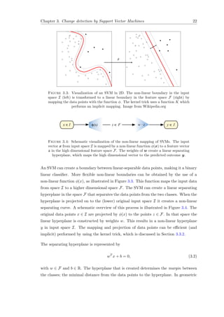
Figure 3.5: Illustration of the separating hyperplane of an SVM. Here w is the nor-
mal vector for the separating hyperplane and size of the margin is 2
w . Image from
Wikipedia.org
sense, w is the normal vector indicating the direction of the hyperplane and b
w de-
termines the offset of the hyperplane from the origin. Since the size of the margin is
equal to 2
w , the maximum-margin hyperplane is found by minimizing w . The data
points which lie on the boundary of the margin are the support vectors. This geometrical
interpretation is illustrated in Figure 3.5. All data points for which yi = −1 are on one
side of the hyperplane and all other data points (for which yi = 1) are on the other side.
The minimal distance from a data point to the hyperplane is equal for both classes.
Minimizing w results in a maximal margin between the two classes. Thus, the SVM
searches for a maximal separating hyperplane.
With every classification method there is a risk of overfitting. In that case the random
error or noise of the data set is described instead of the underlying data. The SVM
classifier can use a soft margin by allowing some data points to lie within the margin,
instead of on the margin or farther away from the hyperplane. For this it introduces
slack variables ξi for each data point and the constant C > 0 determines the trade-off
between maximizing the margin and the number of data points within that margin (and
thus the training errors). The slack variables are a generalization to minimize the sum of
deviations, rather than the number of incorrect data points [18]4. The objective function
for an SVM is the following minimization function:
4
if ξi is chosen to be an indicator function, it still minimizes the number of incorrect data points.](https://image.slidesharecdn.com/593e322b-ac24-4819-ab2f-7f19350bcfbc-160327175441/85/thesis-33-320.jpg)
![Chapter 3. Change detection by Support Vector Machines 24
min
w, b, ξi
w 2
2
+ C
n
i=1
ξi (3.3)
subject to:
yi(wT
φ(xi) + b) ≥ 1 − ξi for all i = 1, . . . , n
ξi ≥ 0 for all i = 1, . . . , n
(3.4)
This minimization problem can be solved using Quadratic Programming (QP) and scales
in the number of dimensions d, since w ∈ Rd. In its dual formulation, as shown in
Equation (3.5), the non-negative Lagrange multipliers αi are introduced. Using this
formulation the problem scales in the number of data points n, since α ∈ Rn. Solving
this problem directly in the high dimensional feature space F makes it intractable. It
is shown that solving the dual formulation is equivalent to solving the primal form [18].
The linear classifier decision function in the dual form is optimized over αi:
f(x) = sgn(
n
i=1
{αiyiK(x, xi) + b}), (3.5)
where K(x, xi) = φ(x)T φ(xi) is the dot product of data objects in feature space F (which
is further discussed in Section 3.3.2). Here every data point in I for which ai > 0 is
weighted in the decision function and thus “supports” the classification machine: hence
the name “Support Vector Machine”. Since it is shown that under certain circumstances
SVMs resembles sparse representations [26, 59], there will often be relatively few La-
grange multipliers with a non-zero value.
Using this formulation two important properties arise [23]:
1. Searching for the maximum margin decision boundary is equivalent to searching
for the support vectors; they are the training examples with non-zero Lagrange
multipliers.
2. The optimization problem is entirely defined by pairwise dot products between
training examples: the entries of the kernel matrix K.
An effect of the first property, combined with the equality to sparse representations, is
that SVMs often have good results, even in the case of high dimensional data or limited
training examples [18]. The second property is what enables an powerful adaptation of
SVMs to learn non-linear decision boundaries. The workings of the kernel matrix K and
the non-linear boundaries are discussed in the following section.](https://image.slidesharecdn.com/593e322b-ac24-4819-ab2f-7f19350bcfbc-160327175441/85/thesis-34-320.jpg)
![Chapter 3. Change detection by Support Vector Machines 25
3.3.2 Kernels
In the previous section, the mapping function φ(x) and the kernel function K were briefly
mentioned. The decision function in Equation (3.5) only relies on the dot products of
mapped data points in the feature space F (i.e. all pairwise distances between the data
points in that space). It shows [23] that for any function K that corresponds to a dot
product in feature space F, without an explicit mapping to the higher dimension F,
the dot products can be substituted by that kernel function K. This is introduced by
Aizerman et al. [1] and applied to Support Vector Classifiers (SVCs) by Vapnik [71],
known as the ‘kernel trick’:
K(x, x ) = (z · z ) = φ(x) · φ(x ) (3.6)
where vectors z and z are projections of data objects x and x through φ(x) on the
features space F. Note that the evaluation of dot products in the feature space F
between vectors is performed indirectly via the evaluation of the kernel K between
(support) vectors in the input space I. This is gives the SVM the ability to create
non-linear decision function without high computational complexity.
The kernel function K can have different forms, such as linear, polynomial and sigmoidal
but the most used (and flexible) form is the Gaussian Radial Base Function (RBF). The
inner product kernel with RBF basis functions have the form
K(x, x ) = exp −
x − x 2
2σ2
, (3.7)
where σ defines the Gaussian width and x − x 2 is the dissimilarity in Euclidean
distance.
The kernel K maps input space I to the feature space F which is a Reproducing Kernel
Hilbert Space (RKHS) of (theoretically) infinite dimensions. As Smola et al. [59] state,
this Gaussian kernel yields good performance, especially when no assumptions can be
made about the data. As an explanation, they show a correspondence between learn-
ing SVMs with RBF kernels and regularization operators. This may give insights in
why SVMs have been found to exhibit high generalization ability (by learning with few
training objects).
The width parameter σ is equal for all kernel functions and is set a priori and determines
the flexibility and complexity of the boundary. In Section 3.3.5 this (hyper)parameter
for an SVM is further discussed.](https://image.slidesharecdn.com/593e322b-ac24-4819-ab2f-7f19350bcfbc-160327175441/85/thesis-35-320.jpg)
![Chapter 3. Change detection by Support Vector Machines 26
The mapping from input space I to F via φ(x) is subject to some continuity assumptions.
This general assumption in pattern recognition, states that two near objects in feature
space should also resemble each other in “real life” [63]. Thus, objects which are close
in feature space should be close in the original input space. When this assumption does
not hold, the example objects would be scatter through the feature space and finding a
decision function becomes very complex.
3.3.3 ν-Support Vector Machine
The first of the OC-SVM methods we will discuss is often referred to as ν-SVM and
introduced by Sch¨olkopf et al. [58]. Instead of estimating the density function of an
distribution P, it focuses on an easier problem: the algorithm finds regions in the input
where the “probability density lives”. This results in a function such that most of the
data is in the region where the function is non-zero.
The constructed decision function f(x) resembles the function discussed in Section 3.3.1.
It returns the value +1 in a (possibly small) region capturing most of the data points,
and −1 elsewhere. The method maps the data points from input space I to a feature
space F (following classical SVMs). In that space the data points are separated from
the origin by a hyperplane, with maximal margin. Since the mapping to the feature
space is based on dot products of the data points, outlier objects (which are dissimilar
from the training set) will be closer to the origin. Thus, maximizing the distance from
the hyperplane to the origin increases the discriminating ability of the decision function.
Furthermore, it holds an intuitive relationship with the classical two-class SVM.
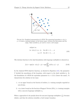
For a new data points x, the function value f(x) determines whether the data point is
part of the distribution (i.e. the value is +1) or a novelty (i.e. the value is −1). The
hyperplane is represented by g(x) = w · φ(x) + ρ = 0 and the decision function is
f(x) = sgn(g(x)). This hyperplane and the separation from the origin is illustrated in
Figure 3.6.
The objective function to find the separating hyperplane is the following minimization
function, which can be solved using QP:
min
w, ξi, ρ
w 2
2
+
1
νn
n
i=1
ξi − ρ (3.8)](https://image.slidesharecdn.com/593e322b-ac24-4819-ab2f-7f19350bcfbc-160327175441/85/thesis-36-320.jpg)
![Chapter 3. Change detection by Support Vector Machines 28
ξi
x
y
R
ξi / |w|
x
y
ρ / |w|
Figure 3.7: Graphical representation of the difference between ν-SVM (left) and
SVDD (right). Note that for the sake of simplicity the kernel functions are not applied.
This method creates a hyperplane, characterized by w and ρ, that separates the data with
maximal margin from the origin in the feature space F. In the following section we will
discuss an alternative method, which uses an circumscribing hypersphere to characterize
the training data. The region inside the hypersphere indicates the region S where the
probability that a data point drawn from P is equal to ν.
3.3.4 Support Vector Data Description
The method introduced by Tax and Duin [64], known as Support Vector Data Descrip-
tion, follows a spherical instead of planar approach. The boundary, created in feature
space F, forms a hypersphere around the (high density region of the) data. The volume
of this hypersphere is minimized to get the smallest enclosing boundary. The chance
of accepting outlier objects is thereby also minimized [67]. By allowing outliers using
slacks variables, in the same manner as classical SVM and ν-SVM, a soft margin is
constructed.
The constructed hypersphere is characterized by the center a and radius R > 0 as
distance from the center to (any data point that is a SV on) the boundary, for which the
volume, and thus the radius R, will be minimized. The center a is a linear combination
of the support vectors. Like the classical SVM and SVDD it can be required that all the
distances from the data points xi to the center a are strict less than R (or equivalent
measure). A soft margin can be allowed by using slack variables ξi. In that case,
the penalty is determined by C and the minimization is expressed as Equation (3.11).
This principle is illustrated in the right image or Figure 3.7. Instead of a separating
hyperplane, constructed by ν-SVM and illustrated on the left of the Figure, the SVDD
creates a hypersphere (in the illustration a circle) around the data points. By using
kernel functions (e.g. the RBF) the hyperspheres in the high dimensional feature space
F corresponds to a flexible and tight enclosing boundary in input space I. Possible](https://image.slidesharecdn.com/593e322b-ac24-4819-ab2f-7f19350bcfbc-160327175441/85/thesis-38-320.jpg)
![Chapter 3. Change detection by Support Vector Machines 29
resulting closed boundaries are illustrated in Figure 3.8. This enclosing boundary is
obtained by minimizing the following error function L which contains the volume of the
hypersphere and the distance from the boundary to the outlier objects:
L(R, a, ξ) = R2
+ C
n
i=1
ξi (3.11)
subject to:
xi − a 2
≤ R2
+ ξi for all i = 1, . . . , n
ξi ≥ 0 for all i = 1, . . . , n
(3.12)
In the dual Lagrangian formulation of this error function L the multipliers α are maxi-
mized:
L =
i
αi(xi · xi) −
i,j
αiαj(xi · xj) (3.13)
subject to:
0 ≤ αi ≤ C,
i
αi = 1
(3.14)
In the maximization of Equation (3.13) a large fraction of the multipliers αi become
zero. The small fraction for which αi > 0 are called the SVs and these objects lie on the
boundary of the description. The center of the hypersphere only depends on this small
number of SVs and the objects for which αi = 0 can be discarded from the solution.
Testing the membership of a (new) object z is done by determining if the distance to
the center a of the sphere is equal or smaller to the radius R:
z − a 2
= (z · z) − 2
i
αi(z · xi) +
i,j
αiαj(xi · xj) ≤ R2
(3.15)
As with Equation (3.5), the solution of this equation only relies on dot products between
the data points in x and z. This means that the kernel projection and trick, as discussed
in Section 3.3.2, can be applied to SVDD as well [64, 66].
Because the Gaussian RBF often yields good (i.e. tight) boundaries, this set of kernels
functions is commonly used:
(x · y) → K(x, y) = exp −
x − y 2
σ2
(3.16)](https://image.slidesharecdn.com/593e322b-ac24-4819-ab2f-7f19350bcfbc-160327175441/85/thesis-39-320.jpg)
![Chapter 3. Change detection by Support Vector Machines 30
Figure 3.8: The SVDD method trained on a banana-shaped data set with different
sigma-values for the RBF kernel. Solid circles are support vectors, the dashed line is
the boundary. Image by Tax [63].
Using this kernel function, the Lagrangian error function L of Equation (3.13) changes
to:
L = 1 −
i
α2
i −
i=j
αiαjK(xi, xj) (3.17)
Using Equation (3.15), the following kernel formulation needs to hold for a new object
z to lie within the hypersphere:
i
αiK(z, xi) ≤
1
2
1 − R +
i,j
αiαjK(xi, xj)
(3.18)
When the Gaussian RBF kernel is applied, and in case the data is preprocessed to
have unit length (for the ν-SVM solution), the two different OC-SVM implementations
ν-SVM and SVDD are shown to have identical solutions [57, 66]
3.3.5 SVM model parameters
SVM-model selecting and tuning depends on two type of parameters [18]:
1. Parameters controlling the ‘margin’ size,
2. Model parameterization, e.g. the kernel type and complexity parameters. For the
RBF kernel the width parameter determines the model complexity.
In case of a RBF kernel, the width parameter σ determines the flexibility and complexity
of the boundary. The value of this parameter greatly determines the outcomes of the
algorithm (e.g. SVDD) as illustrated in Figure 3.8. With a small value for the kernel
width σ, each data point will tend to be used as a support vector (for almost all αi >
0) and the SVDD solution resembles a Parzen density estimation. For large values
of σ, the solution will resemble the original hypersphere solution (in contrast with a
tight boundary around the data). With a large value for the width σ, the boundary
approximates the spherical boundary. The influence of the σ parameter on the SVDD
solution is illustrated in Figure 3.9.](https://image.slidesharecdn.com/593e322b-ac24-4819-ab2f-7f19350bcfbc-160327175441/85/thesis-40-320.jpg)
![Chapter 3. Change detection by Support Vector Machines 31
x
y
σ = small
x
y
σ = medium
x
y
σ = large
Figure 3.9: The SVDD method trained on a banana-shaped data set with different
σ-values for the RBF kernel. Solid circles are support vectors, the dashed line is the
boundary.
As discussed in Section 3.3.3, the SVM parameter C (or ν in case of ν-SVM) is of high
influence on the “smoothness” of the decision function. It acts as an upper bound to
the fraction of outliers and as a lower bound to the fraction of SVs. A more detailed
discussion of the influence of the SVM model parameters can be found in Section 9.8 of
[18] and Section 7.4 from [23]. A detailed discussion of the ν and kernel parameters can
be found in [57].
The following chapter will discuss our proposed method, which incorporates the SVDD
algorithm. It relates the OC-SVM model construction to outlier detection and eventually
change detection, leading to finding a temporal segmentation of time series data.](https://image.slidesharecdn.com/593e322b-ac24-4819-ab2f-7f19350bcfbc-160327175441/85/thesis-41-320.jpg)
![Chapter 4
Application to Human Activity
Time Series Data
This chapter will introduce our method, which we named OCS-HATS [73], and setup for
the temporal segmentation of human activities, using an OC-SVM approach. It shows
our method to apply a OC-SVM based temporal segmentation method to inertial sensor
time series data, often used in the context of Human Activity Recognition. As far as we
know it is the first in its kind, especially on the application of SVDD and SVCPD to real-
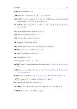
world HAR data. The setup follows the structure as illustrated in Figure 4.1 and further
discussed in Section 4.1. It starts with the data collection phase, in which we both use
artificial and real-world data. The data sets are discussed in Section 6.2. After (optional)
pre-processing, the SVDD algorithm is used to create a model representation, which is
2. Pre-processing
a) Align sensor streams
b) Normalize sensor streams
3. Initialize SVDD model 4. Model updating
Extract properties
Radius Outliers
Indication of change
Ratio-
Thresholding
CuSum
5. Interpret properties
6. Post-processing
1. Data Gathering
Real-world data
Magnetic fieldRotationAccelerometer
Artificial data
Takeuchi & Yamanishi Camci
7. Change points
Figure 4.1: Schematic overview of the change detection method. The first step is
the data gathering, described in Section 4.2. Ater the pre-processing, the data is used
to construct a SVDD model, as described in Section 4.3. Section 4.4 describes which
features of the model are used for the final change indication algorithm, discussed in
Section 4.5.
32](https://image.slidesharecdn.com/593e322b-ac24-4819-ab2f-7f19350bcfbc-160327175441/85/thesis-42-320.jpg)
![Chapter 4. Application to Human Activity Time Series Data 33
iteratively updated. In Section 4.3 this construction phase is discussed and shows the
windowed approach. From this constructed model we can extract some features. In our
case, we use the approximated radius R of the hypersphere to detect changes. Section 4.4
goes into detail about the rationale of using that feature. Finally, in Section 4.5 we
discuss two different, but simple, methods to detect changes in the time series data,
based on the extracted radius R.
4.1 Algorithm overview
The proposed method of this thesis follows the unifying framework as introduced by
Takeuchi and Yamanishi [62] and an similar implementation by Camci [13] with SVMs.
The unifying framework relates the detection of outliers with change points and divides
the whole process in two stages. The first stage determines the outliers in a time series
by giving a score based on the deviation from a learned model, and thereby creates a
new time series. The second stage runs on that new created time series and calculates
an average over a window of the outlier scores. The problem of change detection is
then reduced to outlier detection over that average-scored time series. This method is
named changeFinder by the authors. The implementation by Camci, which uses SVMs
to detect changes is named Support Vector based Change Point Detection.
Whereas changeFinder uses a two-stage probability based algorithm, our approach fol-
lows SVCPD by constructing an SVM over a sliding window. The SVCPD algorithm uses
the location of new data points in the feature space F with respect to the hypersphere
and the hypersphere’s radius R to determine whether the new data point represents a
change point. Our approach is a slight simplification of the algorithm: we only use the
updated model properties (i.e. the radius R) to detect a change. The SVCPD also tests
every new data point with the current modeled hypersphere, to indicate whether it is
an outlier. This difference is further discussed and justified in Section 4.5.
This section gives a description of the method used for the experiments and change
detection mechanism. First described is the method to process the gathered sensor
data. A schematic overview is given in Figure 4.1 and shows the steps of the method. A
more detailed explanation of the “Update model” step is given in the remainder of this
section.
As graphically represented in Figure 4.1, the change detection method starts by process-
ing the data from sensor, such as the accelerometer, magnetic orientation, and rotation
metrics.](https://image.slidesharecdn.com/593e322b-ac24-4819-ab2f-7f19350bcfbc-160327175441/85/thesis-43-320.jpg)
![Chapter 4. Application to Human Activity Time Series Data 34
The first step is to process the raw streams of data originating from a multiple of sensors.
The two processes applied are alignment and normalization. Due to noisy sampling, not
all the timestamps in the data streams are sensed at the same timestamp. Since the
SVDD method requires all the data stream at every timestamp and can not handle
missing data on one of the timestamps, all the unique timestamps are filtered out.
Whilst this results in an overall filtering effect, in practice between 1% and 5% of each
data stream is discarded. The effect of this filtering is not significant and the data is
not modified.
Due to the nature of the sensor signals, a normalization step is required in order to set
the weight for all the data streams equal. The range of the accelerometer signal typically
spans −20 to 20 m/s2, the magnetic field from −60 to 60 µT and the rotations value
range is from −1 to 1. This means that a relative small change in the accelerometer
stream could have a much larger impact on the model than the same (absolute) change
in the rotation stream, whilst the latter has a larger relative impact. The normalization
step ensures that all data is weighted equally and changes in the data are all proportional.
In step 3 the SVDD model is initialized. The first full window over the data stream
is used to construct an initial model. During the initialization the parameters for the
SVDD are provided, begin the kernel type (radial), RBF with σ and the outlier-fraction
C.
Step 4 is executed for every step-size s data points in the stream. Every update the
oldest s data points are removed from and s new data points are added to the SVDD
model. The Incremental Support Vector Data Description (I-SVDD) algorithm by Tax
and Duin [66] is used for efficient incremental model updating. The model is (partially)
reconstructed and new model properties, such as the radius of the hypersphere, is the
result of this step 1.
This final step of this method, step 5, is the interpretation of the model properties.
Many algorithms can be used for this process, all which take a one-dimensional time
series as input and determine where change has occurred. In our setup we used the
Ratio-Thresholding (RT) and CUSUM methods, to show the modularity of this step.
This final step is further discussed in Section 4.5.
1
Other measures are also possible, for instance the distance from all the outliers to the boundary of
the hypersphere or the number of outliers](https://image.slidesharecdn.com/593e322b-ac24-4819-ab2f-7f19350bcfbc-160327175441/85/thesis-44-320.jpg)
![Chapter 4. Application to Human Activity Time Series Data 35
4.2 Data Gathering
In this section we briefly discuss the different data gathering methods used for the change
detection algorithms and experiments. Section 4.2.1 discusses the artificial data sets we
will use. In Section 4.2.2 an overview of the real-world data sets used is provided. Both
sections refer to Chapters 5 and 6 for more details, respectively.
4.2.1 Artificial data
In order to provide an objective, quantitative, comparison to other methods, we will
use artificial data sets which are also used in the earlier work on which OCS-HATS is
based. These are the data sets used by Takeuchi and Yamanishi [62] and Camci [13].
Both construct a collection of one-dimensional time series data according to a second
order Autoregressive (AR) model:
xt = a1xt−1 + a2xt−2 + t. (4.1)
Over the different data series the mean and variance of the Gaussian random variable t
differs and changes at pre-determined change points. Using this data set an quantitative
quality measure over the change detection methods can be obtained and compared. All
the used data sets are listed and analyzed in Chapter 5.
4.2.2 Real-world data
In the second type of data sets we apply our method for change detection and temporal
segmentation to real-world data sets. We record the activities of humans in real-world
environments, both in- and outdoor. Activities performed include sitting, standing,
walking, running in a straight and curved line, and walking up- and downstairs. OCS-
HATS uses the signals from the accelerometer, magnetic field, and rotation sensors.
These time series data are used to detect change points. A video recording from the
performed activity is used to annotate the time series with real change points. The
discovered change points are compared with these annotated change points to give a
qualitative quality measure. In Chapter 6 we give a detailed analysis of the performed
activities and the recorded data sets.
For the experiments we used a smartphone with inertial sensors as recording device.
The activities were recorded using a free Android application Sensor Logger2. This
application was chosen for its convenient data format of the sensor recording and its
2
https://play.google.com/store/apps/details?id= com.kzs6502.sensorlogger](https://image.slidesharecdn.com/593e322b-ac24-4819-ab2f-7f19350bcfbc-160327175441/85/thesis-45-320.jpg)
![Chapter 4. Application to Human Activity Time Series Data 36
Table 4.1: Measured sensor metrics. The set of axis is always the triple (x, y, z)
direction.
Sensor metric Description Units of measure Typical range
Accelerometer Acceleration force along
each axis (including
gravity).
m/s2 −20 – 20
Gravity Force of gravity along each
axis.
m/s2 −10 – 10
Gyroscope Rate of rotation around
each axis.
rad/s −15 – 15
Light Light sensitive sensor at
the front of the phone.
0 – 10000
Linear acceleration Acceleration force along
each axis (excluding
gravity).
m/s2 −20 – 20
Magnetic field Geomagnetic field strength
along each axis.
µT −60 – 60
Orientation Degrees of rotation around
the three physical axis.
Degrees −100 – 360
Rotation Measure of rotation
around the device’s
rotation axis.
Unitless −1 – 1
regularity of the sampling interval. Table 4.1 lists all the recorded metrics. For our
experiments we used the data for the accelerometer, magnetic field and rotation.
We implemented our algorithm in Matlab. For the SVDD model construction phase
we used the dd tools library by Tax [68], which depends on the PR tools package,
originating from the book by Van Der Heijden et al. [69]. Alternatively, the widely used
LibSVM [15] add-on for the SVDD algorithm by Chang et al. [16] can be used.
4.3 Model Construction: Incremental SVDD
After the data is collected (or in the case of the artificial data sets: generated), we con-
struct an online incremental sliding window algorithm. We follow the SVCPD method
by Camci [13] and the I-SVDD implementation by Tax and Laskov [67]. The latter
algorithm combines the techniques of online, unsupervised, and incremental learning
methods with the earlier introduced OC-SVM algorithm SVDD. The method is initial-
ized with a fixed window length and then at every step a new data object is added to and
the oldest data object is removed from this working set. The model construction phase](https://image.slidesharecdn.com/593e322b-ac24-4819-ab2f-7f19350bcfbc-160327175441/85/thesis-46-320.jpg)
![Chapter 4. Application to Human Activity Time Series Data 37
can be regarded as the first stage of the unifying framework by Takeuchi and Yamanishi
[62].
Using the following abstract form of the SVM optimization problem, the extension of
the incremental SVM to the SVDD can be carried out:
max
µ
min
0≤x≤C
aT x+b=0
: W = −cT
x +
1
2
xT
Kx + µ(aT
x + b), (4.2)
where c and a are n × 1 vectors, K is a n × n matrix and b is a scalar. The SVDD
implementation of this abstract form is set by the parameters c = diag(K), a = y and
b = 1. The procedure for the incremental version has two operations for a data object
k: add to and remove from the working set. When a data object k added, its weight xk
is initially set to 0. In case of an object removal, the weight is forced to be xk = 0. Both
the operations conclude with the recalculation of µ and the weights x for all the objects,
in order to obtain the optimal solution for the enlarged or reduced data set. These two
operations are the basis for I-SVDD. With the data points ordered by timestamp, new
data objects are added to and old data objects are removed from the working set.
The size of the initial window of data objects has a lower bound determined by the
hyperparameter C (Equation (3.11)). Because of the equality constraint n
i=1 aixi = 1
and the box constraint 0 ≤ xi ≤ C, the number of objects in the working set must
be at least 1
C . Thus the algorithm is initialized by selection the first 1
C objects for
the working set. In every loop of the algorithm the number of elements added are at
least enough to keep 1
C objects in the window, after removing the oldest objects. The
optimality of the algorithm is proved by analysis of the Karush-Kuhn-Tucker (KKT)
conditions [67].
From experiments it shows that the (online) I-SVDD method results in less false alarms
than the static SVDD. An explanation for this is that I-SVDD follows the changing data
distribution, i.e. small changes over time. Such changes are a drift in mean or increase
in frequency. The I-SVDD algorithm continuously re-models the SVM representation.
This re-modeling of the SVM representation is beneficial for our purpose, since we are
only interested in sudden changes between activities. The following section will discuss
the features extracted from the constructed OC-SVM model at every loop-step of the
algorithm, and Section 4.5 describes how these features are used to detect change.](https://image.slidesharecdn.com/593e322b-ac24-4819-ab2f-7f19350bcfbc-160327175441/85/thesis-47-320.jpg)
![Chapter 4. Application to Human Activity Time Series Data 38
4.4 Model Features
In the previous section we have discussed the I-SVDD method, which creates a OC-SVM
representation of a working set of data objects at every step of the algorithms loop. This
section shows how we interpret the constructed model and extract features to obtain a
measure which can be used for an indication of change points. The next section discusses
how this obtained measure is used to indicate change.
The I-SVDD algorithm creates a spherical OC-SVM representation of the working set
at every step of the algorithm. This model is obtained by the minimization of Equa-
tion (3.11), which incorporates the radius R of the sphere and the distances ξ from the
outliers to the boundary. We will use the radius R of the hypersphere as an indication
of change.
In [66] Tax and Duin provide an analysis of the error of the SVDD algorithm. This error
is based on 1) the fraction fT− of target objects that is rejected, and 2) the fraction
fO+ of outliers that is accepted. Since in OCC situations typically there are (almost) no
examples of outlier objects, Tax and Duin construct a method to generate outliers based
on the assumption that the the location of (potential) outliers are uniformly distributed
around the target set. To minimize the error, calculated by the fractions fT− and fO+, we
should minimize the volume of the target data description (i.e. the boundary of SVDD).
That is because the fraction of accepted outliers fO+ is an estimate of the volume
of the target data description, with respect to the volume of the outlier distribution.
Tax and Duin provide a method to optimize the parameters of the SVDD method,
i.e. the trade-off parameter C and the RBF kernel width σ. This optimization will
result in the modification of the radius R of Equation (3.11) and affects the Lagrangian
inequality (3.18).
Since in our method the parameters C and σ are kept constant, and thereby also the
fraction of target objects being rejected, the only free parameter is the radius R. During
the I-SVDD algorithm the volume of the hypersphere is minimized. This means that
only the radius of the sphere will change during the analysis over the time series data.
We will interpret changes in the radius R with the same continuity assumptions as
mentioned in Section 3.3.2.
For instance, consider two hyperspheres that model two different, but partially overlap-
ping, working sets of objects. If the radius size of these two hyperspheres are close to
each other, that means the distribution of objects in the sets are also similar. In other
words, if the distribution over objects in a working set changes, so does the characteris-
tics of the set, and the radius R of the hypersphere will also change. If in the case of a
change in distribution the data objects in the working set become more heterogeneous,](https://image.slidesharecdn.com/593e322b-ac24-4819-ab2f-7f19350bcfbc-160327175441/85/thesis-48-320.jpg)
![Chapter 4. Application to Human Activity Time Series Data 39
edcba
Time series data
Expected Radius
Figure 4.2: Expected behavior of the radius R of the hypersphere. The upper part
shows a typical sinusoidal time series signal. The lower graph visualizes an abstract
expectation of the values of R. Five possible time windows are illustrated. Windows a,
c and e cover an area of homogeneous signal. The expected value of R is low. The other
two windows, b and d cover a change entering and leaving the window, respectively. At
these locations the radius R is expected to increase temporarily.
the radius of the hypersphere will increase. When, instead, the data objects change
from a heterogeneous set to a more homogeneous, we expect the radius to decrease in
value, since the data objects are closer to each other in the feature space. This relation
between the signal and expected radius R is illustrated in Figure 4.2. It shows that in
the two time windows that cover a heterogeneous set of data objects, the radius of the
hypersphere is expected to be relatively high.
With the I-SVDD algorithm we have effectively implemented a form of dimensionality
reduction by feature extraction, using the radius R. The following section discusses the
algorithms which can be applied to the extracted radius R as a volume estimate. We
thereby follow the setup of the unifying framework by Takeuchi and Yamanishi [62], of
which this section described the first stage.
4.5 Change Detection
In the previous sections we have discussed what data is used for the model construction,
and how that model is interpreted in the context of change detection. We have shown
how the multi-dimensional signal is reduced to a single dimension time series data, based
on the extracted radius R from the constructed hypersphere. This metric is used to
discover changes in the underlying data generation process. We argued that in the case
the data objects set becomes more heterogeneous, we expect an increase in the radius
R. In the same manner we expect that when the change is in the oldest data objects of
the working set, the radius R will decrease, since the data becomes more homogeneous.
An abstract representation of these expectations is illustrated in Figure 4.2.](https://image.slidesharecdn.com/593e322b-ac24-4819-ab2f-7f19350bcfbc-160327175441/85/thesis-49-320.jpg)
![Chapter 4. Application to Human Activity Time Series Data 40
In this section we discuss the methods applicable to the extracted radius R of the
hypersphere, in order to discover a change in the underlying distribution properties.
It is the second stage of our algorithm, analogue to the second stage of the unifying
framework by Takeuchi and Yamanishi [62]. It is also based on the SVCPD method by
Camci [13], although we have simplified the algorithm.
In the SVCPD the first step for a new data point z is to check whether the data point
lies within the enclosing (hyperspherical) boundary of the constructed model. This will
label the new data point as an in- or outlier, relative to the current data set. Depending
on that outcome, the model is updated to include the new data point. The second
step is to inspect the (changed) model properties, i.e. the radius R. In OCS-HATS we
only employ the second step: the inspection of the radius R. We regard the first step
(determine if z is an outlier) to be superfluent: in case it is an outlier, the model update
step will change the radius R in order to let the boundary include the new data point z.
Would the new data object z be already an inlier, then the updated model would not
have a significant change in radius R. Our algorithm is outlined in Algorithm 1.
Algorithm 1 One-Class SVM Human Activity Temporal Segmentation algorithm.
Input: time series X, window size n, thresholds thlow and thhigh, proximity factor δ
Output: collection change points
1: change points ← empty collection
2: radii ← empty collection
3: Initialize w ← incremental svdd with first n samples from x
4: while new sample x from X at time t do
5: Add x to w
6: sphere ← update hypersphere(w)
7: radius ← extract radius(sphere)
8: radii[t] ← radius
9: ← calculate ratio from previous average radii and current radius
10: if < thlow or > thhigh then
11: Add current time t to change points
12: Empty previous radii
13: end if
14: Remove oldest x from w
15: end while
16: Merge cp based on proximity δ
The problem of change detection in complex multi-dimensional time series is now reduced
to finding change in a one-dimensional time series. Besides the dimensionality reduction,](https://image.slidesharecdn.com/593e322b-ac24-4819-ab2f-7f19350bcfbc-160327175441/85/thesis-50-320.jpg)
![Chapter 4. Application to Human Activity Time Series Data 41
the form of the signal is also simplified. Whereas the original signal was represented as
a sinusoidal or second order AR model, the new time series is of much simpler form. In
our method we leave open the precise method which is used to find change points in
the obtained change indication values. Below, we will gives two examples of methods
which can be applied. The first is a family of methods based on the CUSUM method.
The second example is a ratio-based thresholding mechanism used by Camci [13]. We
conclude this section by discussing some post-processing techniques we have used, to
decrease the number of false positives.
4.5.1 CUSUM based methods
Many of the simple change detection methods are based on CUSUM, originally intro-
duced by Page [54]. Other variations and extensions of the method are proposed and
used ([3, 37, 38]). Here we will discuss the simple form, which only detects changes as
an increase in value of the examples, in this case the radius R. The cumulative sum for
all the values is calculated:
Sn =
n
k=0
Rk (4.3)
and a change is detected when the value of the cumulative sums minus the minimum
encountered exceeds a predetermined threshold h:
Sn − min
0≤i<n
Si ≥ h. (4.4)
Extensions of the CUSUM method have been proposed. Amongst others, extensions
which extend its use to two-threshold methods, and methods appropriate for changes in
mean or variance [38]. Whilst adaptive methods have been proposed [3], most methods
require manual determination of the threshold parameter h.
4.5.2 Ratio-thresholding
The second example of an algorithm that interprets the change indication time series
and transforms it to change detection is the radius ratio thresholding method used by
Camci [13]. The method shares characteristics with CUSUM, since it relies on summa-
tion of historic data and thresholds for change detection. The method calculates the
radius ratio t by taking the ratio of the current radius rt at time t to the average radii
since the last change point y:
t =
rt
mean(ry:t−1)
, (4.5)](https://image.slidesharecdn.com/593e322b-ac24-4819-ab2f-7f19350bcfbc-160327175441/85/thesis-51-320.jpg)
![Chapter 4. Application to Human Activity Time Series Data 42
t1
t2
t3
thhigh
ħt
Figure 4.3: Abstract illustration of the radius ratio thresholding. The peak at t1
generates a single change point. The region between t2 and t3 generates multiple
change points, since the value of t keeps increasing.
where mean(ry:t−1) is the average of the previous approximated radii. By using only
historic data, this method can be incorporated in an online change detection method.
The ratio t is compared with two thresholds: the low threshold thlow and the high
threshold thhigh. When the data objects in the working set become more homogeneous
at time t, the radius R of the hypersphere and thereby the ratio t will decrease. When
the new value of r is lower than the low threshold thlow, a change detection is observed
for time t. The same holds for a more heterogeneous set of data and an increase of r
higher than thhigh. This is illustrated in Figure 4.3.
The appropriate values for the thresholds strongly depend on the characteristics of the
data and the parameter C (as discussed in Section 3.3.4). This trade-off parameter
regulates the fraction of data objects that will be rejected from the constructed model.
Since a high value of C assigns a high penalty to outliers, data objects are more likely
to be incorporated into the hypersphere by increasing the radius. For low values of C
the cost of rejecting data objects is, compared to the benefits of a smaller hypersphere,
relatively low. This gives a relation between the parameters C, thlow, thhigh, and the
sensitivity of the radius ratio based thresholding method. A high value of C, or values
close to 1 for thlow and thhigh result in a sensitive change detection procedure. The
reverse results in less sensitive methods. The correct values for the intended sensitivity
need to be empirically determined.
4.5.3 Post-processing
In our method we use the ratio based thresholding, also used by Camci [13]. From
preliminary experiments we observed that a single change in the data can cause many
detected change points, using the ratio based method. This phenomenon can be ex-
plained by the nature of the thresholding method. Since a single (high or low) threshold
is set for ratio of the radii, high values are considered to be a change point before the
highest point of the peak. As illustrated in Figure 4.3, the peak at t1 represents a single
change point. The region from t2 to t3 is strictly increasing. At t2 a change point is](https://image.slidesharecdn.com/593e322b-ac24-4819-ab2f-7f19350bcfbc-160327175441/85/thesis-52-320.jpg)

![Chapter 5
Artificial data results
In this chapter we will apply the proposed algorithm as stated in the previous chapter
to artificial data sets. For comparison, we use some of the data sets that are used by
Camci [13] and Takeuchi and Yamanishi [62]. These data sets are generated by Gaussian
noise distributions. In Section 5.1 the precise generation method and characteristics of
the data sets are discussed. For our final change detection mechanism we use the RT-
method, also applied by Camci [13]. This is a simple and fast method and allows us to
mainly focus on the OC-SVM model properties that should reflect changes in the data.
The results of these two methods are discussed in Section 5.3.
5.1 Artificial data generation
In this section we present four data sets, as used by Camci [13] and Takeuchi and
Yamanishi [62], to provide for a quantitative performance comparison. All the data sets
are modeled by a second-order AR-model as in Equation (5.1), where t is a Gaussian
distribution modeling the noise with mean 0 and variance σ2 = 1, a1 = 0.6 and a2 =
−0.5.
xt = a1xt−1 + a2xt−2 + t, (5.1)
The length of xt is 10000 and change points are generated at each y × 10000th data
point, with y = (1, 2, 3, . . . , 9).
Using this general AR-model, we create four different data sets, all visualized in Fig-
ure 5.1. Each data set is characterized by a change in mean, variance, or both in the
Gaussian term t:
44](https://image.slidesharecdn.com/593e322b-ac24-4819-ab2f-7f19350bcfbc-160327175441/85/thesis-54-320.jpg)
![Chapter 5. Artificial data results 45
1. Fixed increasing mean: at each change point y the mean is increased with
∆(y) = 5. This set is the first data set of Camci [13]. The main characteristic is
that the difference between the means of the Gaussian term t is fixed and thus
the relative distance becomes smaller. The data is plotted in Figure 5.1a.
2. Reduced increasing mean: at each change point y the mean is increased with
∆(y) = 10 − y. This set is the first data set of Takeuchi and Yamanishi [62]. In
contrast with the previous set, in this set the absolute difference in mean is reduced
over time. The data is plotted in Figure 5.1b.
3. Reduced increasing mean, increasing variance: at each change point y the
mean is increased with ∆(y) = 10 − y and the standard deviation is of t is
0.1/(0.01 + (10000 − x)/1000). This set is the second set of Camci [13]. This
set combines the reduced increasing mean property of the previous set with an
increasing variance, causing the change points to become more vague over time.
The data is plotted in Figure 5.1c.
4. Alternating variance: at each change point y the variance σ2 is set to 9.0 when
y is odd, and to 1.0 otherwise. This set is the thirds sets from Camci [13] and
Takeuchi and Yamanishi [62]. This data set is used to measure the ability of
detecting changes in decrease of variance, as Camci [13] claims is not trivial. The
data is plotted in Figure 5.1d.
5.2 Quality metrics
For an quantitative measure of quality of the proposed method applied to the four
aforementioned data sets, we employ two metrics, inspired by and slightly altered from
Takeuchi and Yamanishi [62]. The first metric is the average delay davg, for which we
first need to define the notion of delay d for each change:
d(y) = |ty − t∗
y|, (5.2)
where ty is the time of the closest discovered change point and t∗
y is the true change
time. We can then define the davg over all the discovered change points Y as:
davg(Y ) =
Y
y=1 d(y)
Y
. (5.3)
Besides the delay, and the standard deviation std(davg) to measure the spread, which
should be low to indicate discovered change points near the actual change point, we](https://image.slidesharecdn.com/593e322b-ac24-4819-ab2f-7f19350bcfbc-160327175441/85/thesis-55-320.jpg)
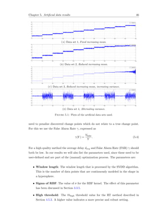
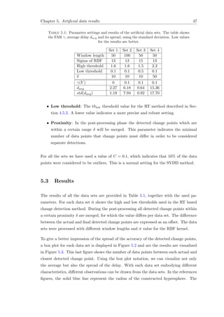
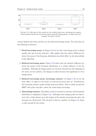
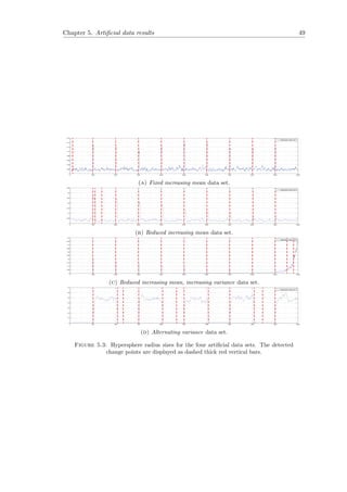
![Chapter 6
Real-world results
In this chapter we discuss the real-world data sets used for this research and the perfor-
mance of our proposed algorithm on these data sets. In Section 6.1 we discuss available
data sets and argue that these are inappropriate for our research. It is followed by an
overview of the setup we have created to record our continuous data sets in a real-world
environment, both for in- and outdoor activities. The series of activities performed are
discussed in Section 6.2. In that section we show typical plots of the inertial sensor
data and stills from the video recordings. That will illustrate the setting in which the
activities are performed and the characteristics of continuous data. The results of the al-
gorithm are discussed in Section 6.3. Finally, we provide a list of possible improvements
in Section 6.4.
The results are measured with both quantitative measures, as introduced in Section 5.2,
and qualitative claims on the performance of the algorithm applied to the real-world
data. Since the data sets used are real-world recordings, we will put emphasis on the
latter type of quality measures i.e. the qualitative claims.
6.1 Data Sets
In the previous chapter we have applied our method OCS-HATS to the artificial data
sets from Camci [13] and Takeuchi and Yamanishi [62]. In this chapter we apply the
method to real-world data sets. The data sets come from inertial sensor data recorded
during human activities, such as walking, running, ascending and descending stairs,
and standing still. To compare our results with other research, we have tried to apply
OCS-HATS to two commonly used data sets. The first is the data from the WISDM
lab [43]. As an excerpt from the data in Figure 6.1 shows, the activities are recorded
50](https://image.slidesharecdn.com/593e322b-ac24-4819-ab2f-7f19350bcfbc-160327175441/85/thesis-60-320.jpg)
![Chapter 6. Real-world results 51
0 100 200 300 400 500 600 700
−15
−10
−5
0
5
10
15
20
Time (s)
Accelerometer
Run Walk
Upstairs UpstairsDownstairs
Figure 6.1: Excerpt from the WISDM data set [43]. The first five activities of subject
33 are displayed. Due to the discontinuous nature of the recordings, this data set can
not be used for change detection.
0 1 2 3 4 5 6 7 8 9
−0.6
−0.4
−0.2
0
0.2
0.4
0.6
0.8
Time (s)
Accelerometer
Standing Standing StandingLaying Laying Laying LayingSitting Sitting Sitting SittingDownstairs Downstairs DownstairsUpstairs UpstairsWalking Walking
Figure 6.2: Excerpt from the UCI HAR data set [5]. The recorded training activities
of subject 25 are displayed. Due to the imprecise (and possibly incorrect) labeling and
the short duration of activities, the data set can not be used for the change detection
method as described in this thesis.
non-continuous. Whilst this data set is convenient for activity classification, it does not
allow for detection of change points. Even if the gap between the activities would be
removed, the transition segments between activities would still be missing and thus the
data set would not reflect continuous recordings. The other commonly used data set is
the UCI HAR from the Machine Learning Repository and originates from [5]. As shown
in an except in Figure 6.2, the labeling to the data segments seems to be incorrect.
Furthermore, it is not clear how the data is recorded and whether all activities are
performed continuously.
Because of the above described shortcomings of commonly used data sets, we have
decided to record activities by ourselves. The following requirements were set for our
data sets:
1. The activities need to be performed and recorded in a continuous manner,
2. The environment should be natural and both in- and outdoor,
3. The data should be clearly annotated, as objective as possible,
4. The required hardware (and software) should be widely available.
With these requirements in mind, we have created the following setup. All activities
were recorded by a smartphone worn on body in the right front pants pocket of the](https://image.slidesharecdn.com/593e322b-ac24-4819-ab2f-7f19350bcfbc-160327175441/85/thesis-61-320.jpg)
![Chapter 6. Real-world results 52
subject. The used phones are the HTC Sensation XE and HTC Desire, running
the Android smartphone operating system. During the activities the inertial sensor
data is recorded using a free application, Sensor Logger. This application records
the sensor data to CSV files, which are then transformed to MATLAB compatible files.
The constructed algorithm processes the data in an online manner (using only current
and historic data). The MATLAB implementation uses the SVDD library dd tools
by Tax [68]. During the activities, the subject is recorded with a video camera to enable
manual labeling and determination of the change points. As illustrated in the top row
of Figure 6.5, the manual labeling is an ambiguous task. In Figure 6.5b a transition
between walking and running is shown. It is impossible to determine the exact location
of the change point and thus quantitative quality measures (such as the delay) are of
less importance.
Using the video recordings, the data sets are manually annotated, as shown in the plots
of Figures 6.3, 6.4 and 6.7. The graphs display each from a single recording the inertial
sensor values (see Table 4.1 for an explanation of the metrics), with manually annotated
activities above the data. The manually and discovered change points are compared to
draw quality conclusions over the algorithm’s performance. All of the used data sets,
including the video material and manual labeling, are made available to the public as
the Almende Continuous Real-world Activities with on-body smartphones Sensors Data
Set (ACRAS) [72] for further research. The following section discusses the performed
activities during the recordings.
6.2 Data Gathering
For our data sets of real-world activities we have sampled both in- and outdoor activities.
The subjects performing the activities are three males, of an age around 25. We have
used four types of recordings. The first type (Run 1 and Run 2) consists of various
outdoor recordings with segments of walking, running and standing. For the second
type (Run 3, 4, and 5) some of the same activities are performed in a straight line,
whilst others are performed around corners or in a wide circular direction. The third
type (Run 6) consists mainly of walking up and down circular shaped stairs, with small
horizontal parts between the segments. The last type is for Run 7, in which we walked
in a straight line, took a 90◦ counter-clockwise turn (around the corner) and continued
walking. A more detailed description of the performed activities follows.](https://image.slidesharecdn.com/593e322b-ac24-4819-ab2f-7f19350bcfbc-160327175441/85/thesis-62-320.jpg)

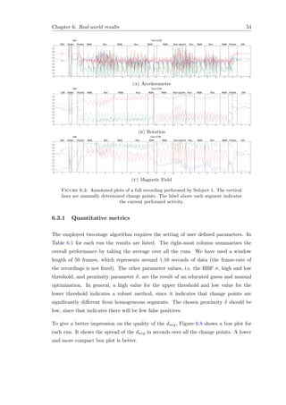
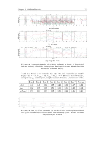
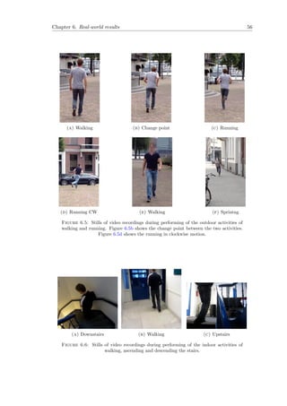
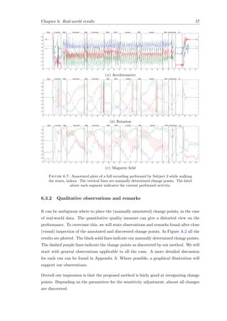
![Chapter 6. Real-world results 58
Our first observation is that with a high sensitivity it seems that the method produces
many false positives. Although the performed activity did not change around those false
positives, there was a change in the recorded data. This is a drawback of the method:
since the sensitivity is set globally, it can produce false positive change points for some
segments of a run.
The second observation is that the method often recognizes a change point before our
annotation. Again, after closer inspection we can see that the data changes shape and
distribution before we annotated a change based on the video recordings. This effect
can be observed in the case of a transition from running to walking; the last ‘steps’ of
running are already labeled as change points. As with the above behavior, this is subject
to parameter settings.
Considering the overall performance and results, we have the following observations:
• Merging: in our method we use a proximity time period δ (usually up to 0.5 -
1.0 seconds) to merge discovered change points that are close together. Multiple
merging-strategies can be applied, and in our method we use the naive implemen-
tation by simply ignoring all the discovered change points that occur less than δ
seconds after the previous change point. This works well when there is a block of
noisy data with a high amount of (falsely) discovered change points. On the flip
side, this method will ignore real new change points which occur during the noisy
period. This problem on itself can be formulated as a change detection problem.
• Masking: Since the parameters for the detection method are set globally, it is
difficult to discover all the change points (and only the change points) without a
high false alarm rate. If a change point is proceeded by a noisy block, then the
real change point will be merged with the previous change points. In an other
case, where a change point is very clear represented in the data but the next near
change point is more subtle, the latter change point is masked by the former. This
masking effect is also discussed in [38], where an iterated approach is applied.
• Variance and threshold levels: For our video synchronization, we started and
ended each recording with a few seconds in which the recording smartphone was
kept still in the air. Then we shake the smartphone to get a sudden change in the
inertial sensor data, so the video and sensor data stream can easily be aligned.
During the still period, the data variance, and thus the constructed hypersphere,
becomes very small. As a results, even small movements are considered to be
changes and in the case of a mid-air kept smartphone a lot of false change points
are detected. Due to the merging effect described above, the final real change
point (shaking the smartphone) is not discovered.](https://image.slidesharecdn.com/593e322b-ac24-4819-ab2f-7f19350bcfbc-160327175441/85/thesis-68-320.jpg)

![Chapter 7
Conclusion
This research has applied OCC methods to inertial sensor data, recorded during the
performance of various human activities, in order to create a temporal segmentation of
those recordings. The goal was to find the change points between activities, assuming
that it will aid our understanding of the sensor values. To do so, we used the SVDD
algorithm by Tax [64] and applied it to a sliding window of data, as done by Camci [13].
From these methods we have created our own method OCS-HATS and made it publicly
available [73], which is a slightly modified implementation of SVCPD by Camci [13]
applied to HAR data. An increase of the radius of the constructed hypersphere, which
encloses the data objects and increases with heterogeneous segments of data, is extracted
and used for indication of change.
In Section 7.1 we will further discuss the proposed method for temporal segmentation
of inertial sensor signals from human activities. Our main findings and contributions
are discussed in Section 7.2. The limitations of our method and research is subject of
Section 7.3. Section 7.4 provides suggestions for future research. Section 7.5 is the final
section of this thesis.
7.1 Proposed method
The goal of this research was to find a temporal segmentation of recordings obtained
from human activities. This was performed in the wider context of activity classifica-
tion. Currently, many algorithms obtain an implicit segmentation as a side-effect of
direct activity classification. In this research the primary goal was finding a temporal
segmentation, which is assumed to be able to aid the classification step. This problem is
reduced to finding change points in temporal data sets originating from inertial sensors.
60](https://image.slidesharecdn.com/593e322b-ac24-4819-ab2f-7f19350bcfbc-160327175441/85/thesis-70-320.jpg)
![Chapter 7. Conclusion 61
We have considered a range of segmentation methods, from which the method by
Camci [13] showed potential. It is based on the detection of outliers in a time se-
ries data, assuming that an increase of outliers indicates a change in the underlying
generating model. For the detection of outliers it uses the SVDD method by Tax [64].
It tests every new data point with the constructed model; whether the data point is in
or outside the model, and whether the model increases or decreases in radius size. The
constructed sliding-window algorithm, SVCPD, is applied to artificial Gaussian noise
data.
In this research we have applied the method by Camci [13] to data from inertial sensors,
recorded by smartphones. We have used the accelerometer data for measurement of
speed, the gyroscope data for measurement of rotation, and the magnetometer to mea-
sure the direction and orientation of the performed activities. The proposed method, as
discussed in Chapter 4, reduces a high dimensional signal to a single property, obtained
from the constructed model, which can be interpreted to indicate change.
The constructed model follows the implementation of Tax and Laskov [67] for an incre-
mental version of SVDD, I-SVDD. This algorithm creates a OC-SVM model by process-
ing the data over a sliding window. The model represents a hypersphere from which the
radius size is extracted. That property is of interest since the assumption is that a het-
erogeneous window of data will show an increase of radius, in relation to a homogeneous
segment of data. The homogeneous segment of data will have a relatively small radius
since the data points will be close together, resulting from the continuity assumptions.
To test our approach, we have used the same data as used in the experiments from
Camci [13] and Takeuchi and Yamanishi [62], for which the results are comparable with
the original research (see Section 5.3). Furthermore, since this research is focused around
human activities, we have recorded and manually annotated in- and outdoor activities.
The discovered change points were compared to the annotated change points, obtained
from video recordings. The results where discussed in Section 6.3. In this research
we found that other public available and wide used common data sets, such as the
WISDM [43] and UCI HAR [5], were not useful for our purpose, since the activities are
non-continuously recorded.
7.2 Contributions
While temporal segmentation of time series data is not uncommon, the application to
inertial signals is currently not under much research attention. For other contexts it
has been applied, such as motion tracking [8, 44]. In the context of human activities](https://image.slidesharecdn.com/593e322b-ac24-4819-ab2f-7f19350bcfbc-160327175441/85/thesis-71-320.jpg)
![Chapter 7. Conclusion 62
the segmentation obtained from inertial sensor signals is often an implicit result of
classification.
We have shown that it is possible to explicitly obtain a temporal segmentation, expressed
as change points, of activities performed by humans. This was performed in a real-world
setting, showing the robustness of the method for noisy data. Since manual labeling (the
annotation of change points on the time series data) of human activities is ambiguous
we put emphasis on the qualitative inspection of the results. The proposed method gives
fairly good results, although parameter tuning is a subject of further research.
We have constructed OCS-HATS as a slightly simplification of SVCPD by Camci [13]
application to real-world inertial sensor data. The Matlab implementation is free to
use for the public [73]. We have tested our proposed method with the same artificial
data and did not find a deterioration in the results. Because of the noisy nature of
the recorded activities and the ability to segment the time series, we have shown that
OCS-HATS is a robust method for real-world applications.
The proposed method is, as far as we know, the first application of OC-SVM based
methods to on-body worn inertial sensor signals, such as accelerometer data. Further-
more, it applies the algorithms, amongst others of Tax and Duin [64], to real-world data.
We have shown that the assumption of a change the performed activity results, due to a
change in the data distribution, in an increase of the hypersphere’s radius. This increase,
and a similar decrease in the case of homogeneous activity distribution in the current
window, can be used for an indication of change.
The proposed OCS-HATS method processes the raw inertial sensor data, originating
from sensors as accelerometers and magnetic field sensors. This contrasts with many
other approaches that extract features in a pre-processing stage.
Furthermore, because the it is an online method, it is suitable for applications that need
direct segmentation of time series data.
The commonly used data sets [5, 43] are recorded in a non-continuous manner. The
proposed method requires data streams of continuous activities. Annotating change
points on this kind of time series can be ambigious, so we needed to have a ground
truth. Because of these two shortcomings, we have recorded continuous real-world data
sets, together with a third persion point of view video stream. All the recorded data is
made publicly available as the ACRAS data set [72]. Using our results as a benchmark,
it is possible for others to use our data set and improve on it.](https://image.slidesharecdn.com/593e322b-ac24-4819-ab2f-7f19350bcfbc-160327175441/85/thesis-72-320.jpg)
![Chapter 7. Conclusion 64
Since temporal segmentation of inertial signal is not yet a very active field of study,
more studies can be performed on this subject. In our approach we have used (all) the
raw data directly, to create a method independent of the domain. In the field of activity
recognition many methods make use of pre-processing steps, from which one step often
is feature extraction from the raw data. That, and other pre-processing steps, could be
incorporated in explicit temporal segmentation of inertial signals. Future research could
focus on using those extracted features to aid the detection of change points.
Similar, feature selection if often used to use only the best dimensions of a signal. We
have encountered situations in which the exclusion of some sensors, e.g. the accelerom-
eter, yields better results. This occurs mainly in situations where a rotation is part of
the change (e.g. walking around a corner). Thus depending on the desired granularity of
the segmentation, it can be beneficial to discard some of the time series data. Applying
feature selection to the sensors to restrict the data used for model construction could be
a subject of further research.
Finally, the application of OC-SVM based methods to new types of data is an interest-
ing subject for further research in itself. It creates a powerful non-linear classification
solution and combined with optimization techniques can reduce problems of relatively
high dimensionality to a single (or a few) dimensions.
7.5 Final words
In this research we have constructed a method to segment inertial sensor time series data,
from performed human activities. To this end we have applied OCC and OC-SVM based
method to our own recorded data sets. We followed the approach by Camci [13] and used
the theory and implementation of SVDD by Tax [63, 68]. Although the performance
of the method heavily depends on user set parameters, the results are promising. We
believe that the temporal segmentation of time series data can aid the process of activity
classification, which is a logical follow-up on this research.
We have created a continuous recorded data set ACRAS [72] from inertial sensors found
in typical modern smartphones. The transition periods between the activities are part
of the time series data. This makes the data set useful for research on segmentation.
Besides the manually annotated change points can the ground truth of the performed
activity be determined by using the provided video recordings of the activities.
With our method for temporal segmentation of human activities, OCS-HATS [73], we
believe to have contributed to the field of machine learning in the context of Human
Activity Recognition.](https://image.slidesharecdn.com/593e322b-ac24-4819-ab2f-7f19350bcfbc-160327175441/85/thesis-74-320.jpg)
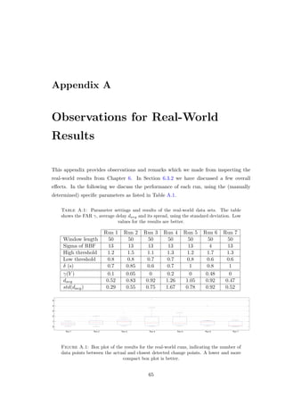
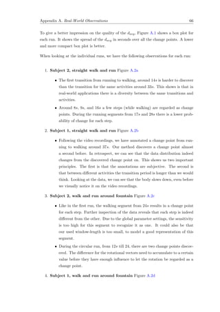
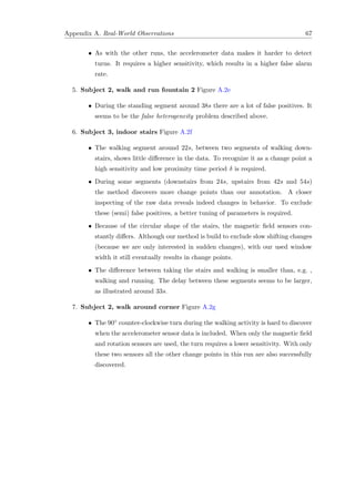
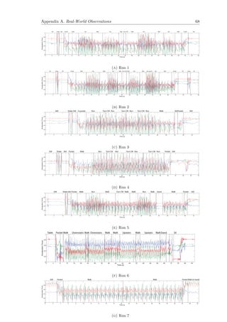
![Bibliography
[1] A Aizerman, Emmanuel M Braverman, and LI Rozoner. Theoretical foundations
of the potential function method in pattern recognition learning. Automation and
remote control, 25:821–837, 1964.
[2] Hirotugu Akaike. A new look at the statistical model identification. Automatic
Control, IEEE Transactions on, 19(6):716–723, 1974.
[3] Cesare Alippi and Manuel Roveri. An adaptive cusum-based test for signal change
detection. In Circuits and Systems, 2006. ISCAS 2006. Proceedings. 2006 IEEE
International Symposium on, pages 4–pp. IEEE, 2006.
[4] Davide Anguita, Alessandro Ghio, Stefano Pischiutta, and Sandro Ridella. A
hardware-friendly support vector machine for embedded automotive applications.
In Neural Networks, 2007. IJCNN 2007. International Joint Conference on, pages
1360–1364. IEEE, 2007.
[5] Davide Anguita, Alessandro Ghio, Luca Oneto, Xavier Parra, and Jorge L Reyes-
Ortiz. Human activity recognition on smartphones using a multiclass hardware-
friendly support vector machine. In Ambient Assisted Living and Home Care, pages
216–223. Springer, 2012.
[6] Akin Avci, Stephan Bosch, Mihai Marin-Perianu, Raluca Marin-Perianu, and Paul
Havinga. Activity recognition using inertial sensing for healthcare, wellbeing and
sports applications: A survey. In Architecture of Computing Systems (ARCS), 2010
23rd International Conference on, pages 1–10. VDE, 2010.
[7] Ling Bao and Stephen Intille. Activity recognition from user-annotated acceleration
data. Pervasive Computing, pages 1–17, 2004.
[8] J. Barbiˇc, A. Safonova, J.Y. Pan, C. Faloutsos, J.K. Hodgins, and N.S. Pollard.
Segmenting motion capture data into distinct behaviors. In Proceedings of Graph-
ics Interface 2004, pages 185–194. Canadian Human-Computer Communications
Society, 2004.
69](https://image.slidesharecdn.com/593e322b-ac24-4819-ab2f-7f19350bcfbc-160327175441/85/thesis-79-320.jpg)
![Bibliography 70
[9] Vic Barnett and Toby Lewis. Outliers in statistical data, volume 3. Wiley New
York, 1994.
[10] M. Basseville, I.V. Nikiforov, et al. Detection of abrupt changes: theory and appli-
cation, volume 104. Prentice Hall Englewood Cliffs, NJ, 1993.
[11] Thomas Bernecker, Franz Graf, Hans-Peter Kriegel, Christian Moennig, Dieter Dill,
and Christoph Tuermer. Activity recognition on 3d accelerometer data (technical
report). 2012.
[12] Robert L Brown, James Durbin, and John M Evans. Techniques for testing the
constancy of regression relationships over time. Journal of the Royal Statistical
Society. Series B (Methodological), pages 149–192, 1975.
[13] Fatih Camci. Change point detection in time series data using support vectors.
International Journal of Pattern Recognition and Artificial Intelligence, 24(01):73–
95, 2010.
[14] F Chamroukhi, S Mohammed, D Trabelsi, L Oukhellou, and Y Amirat. Joint
segmentation of multivariate time series with hidden process regression for human
activity recognition. Neurocomputing, 2013.
[15] Chih-Chung Chang and Chih-Jen Lin. Libsvm: a library for support vector ma-
chines. ACM Transactions on Intelligent Systems and Technology (TIST), 2(3):27,
2011.
[16] Wei-Cheng Chang, Ching-Pei Lee, and Chih-Jen Lin. A revisit to support vector
data description (svdd).
[17] Tsung-Lin Cheng. An efficient algorithm for estimating a change-point. Statistics
& Probability Letters, 79(5):559–565, 2009.
[18] Vladimir Cherkassky and Filip M Mulier. Learning from data: concepts, theory,
and methods. Wiley. com, 2007.
[19] Corinna Cortes and Vladimir Vapnik. Support-vector networks. Machine learning,
20(3):273–297, 1995.
[20] M.O. Derawi. Accelerometer-based gait analysis, a survey. Norsk informasjon-
ssikkerhetskonferanse (NISK), 2010.
[21] R.W. DeVaul and S. Dunn. Real-time motion classifica-
tion for wearable computing applications. 2001, project paper,
http://www.media.mit.edu/wearables/mithril/realtime. pdf, 2001.](https://image.slidesharecdn.com/593e322b-ac24-4819-ab2f-7f19350bcfbc-160327175441/85/thesis-80-320.jpg)
![Bibliography 71
[22] Andr´es Duque, Fco Javier Ord´o˜nez, Paula de Toledo, and Araceli Sanchis. Offline
and online activity recognition on mobile devices using accelerometer data. In
Proceedings of the 4th international conference on Ambient Assisted Living and
Home Care, pages 208–215. Springer-Verlag, 2012.
[23] Peter Flach. Machine learning: the art and science of algorithms that make sense
of data. Cambridge University Press, 2012.
[24] Erich Fuchs, Thiemo Gruber, Jiri Nitschke, and Bernhard Sick. Online segmentation
of time series based on polynomial least-squares approximations. Pattern Analysis
and Machine Intelligence, IEEE Transactions on, 32(12):2232–2245, 2010.
[25] Keinosuke Fukunaga. Introduction to statistical pattern recognition. Access Online
via Elsevier, 1990.
[26] Federico Girosi. An equivalence between sparse approximation and support vector
machines. Neural computation, 10(6):1455–1480, 1998.
[27] E. Guenterberg, H. Ghasemzadeh, V. Loseu, and R. Jafari. Distributed contin-
uous action recognition using a hidden markov model in body sensor networks.
Distributed Computing in Sensor Systems, pages 145–158, 2009.
[28] E. Guenterberg, S. Ostadabbas, H. Ghasemzadeh, and R. Jafari. An automatic
segmentation technique in body sensor networks based on signal energy. In Pro-
ceedings of the Fourth International Conference on Body Area Networks, page 21.
ICST (Institute for Computer Sciences, Social-Informatics and Telecommunications
Engineering), 2009.
[29] Tian Guo, Zhixian Yan, and Karl Aberer. An adaptive approach for online seg-
mentation of multi-dimensional mobile data. In Proceedings of the Eleventh ACM
International Workshop on Data Engineering for Wireless and Mobile Access, pages
7–14. ACM, 2012.
[30] V. Guralnik and J. Srivastava. Event detection from time series data. In Proceedings
of the fifth ACM SIGKDD international conference on Knowledge discovery and
data mining, pages 33–42. ACM, 1999.
[31] Fredrik Gustafsson. The marginalized likelihood ratio test for detecting abrupt
changes. Automatic Control, IEEE Transactions on, 41(1):66–78, 1996.
[32] Wolfgang H¨ardle. Nonparametric and semiparametric models. Springer Verlag,
2004.](https://image.slidesharecdn.com/593e322b-ac24-4819-ab2f-7f19350bcfbc-160327175441/85/thesis-81-320.jpg)
![Bibliography 72
[33] Zhen-Yu He and Lian-Wen Jin. Activity recognition from acceleration data using
ar model representation and svm. In Machine Learning and Cybernetics, 2008
International Conference on, volume 4, pages 2245–2250. IEEE, 2008.
[34] Kathryn Hempstalk, Eibe Frank, and Ian H Witten. One-class classification by com-
bining density and class probability estimation. In Machine Learning and Knowl-
edge Discovery in Databases, pages 505–519. Springer, 2008.
[35] J. Himberg, K. Korpiaho, H. Mannila, J. Tikanmaki, and H.T.T. Toivonen. Time
series segmentation for context recognition in mobile devices. In Data Mining, 2001.
ICDM 2001, Proceedings IEEE International Conference on, pages 203–210. IEEE,
2001.
[36] Victoria Hodge and Jim Austin. A survey of outlier detection methodologies. Ar-
tificial Intelligence Review, 22(2):85–126, 2004.
[37] Chih-Chiang Hsu. The mosum of squares test for monitoring variance changes.
Finance Research Letters, 4(4):254–260, 2007.
[38] Carla Incl´an and George C Tiao. Use of cumulative sums of squares for retrospective
detection of changes of variance. Journal of the American Statistical Association,
89(427):913–923, 1994.
[39] Takafumi Kanamori, Shohei Hido, and Masashi Sugiyama. A least-squares approach
to direct importance estimation. The Journal of Machine Learning Research, 10:
1391–1445, 2009.
[40] Y. Kawahara and M. Sugiyama. Change-point detection in time-series data by direct
density-ratio estimation. In Proceedings of 2009 SIAM International Conference on
Data Mining (SDM2009), pages 389–400, 2009.
[41] E. Keogh, S. Chu, D. Hart, and M. Pazzani. An online algorithm for segmenting
time series. In Data Mining, 2001. ICDM 2001, Proceedings IEEE International
Conference on, pages 289–296. IEEE, 2001.
[42] Shehroz S Khan and Michael G Madden. A survey of recent trends in one class clas-
sification. In Artificial Intelligence and Cognitive Science, pages 188–197. Springer,
2010.
[43] Jennifer R Kwapisz, Gary M Weiss, and Samuel A Moore. Activity recognition
using cell phone accelerometers. ACM SIGKDD Explorations Newsletter, 12(2):
74–82, 2011.](https://image.slidesharecdn.com/593e322b-ac24-4819-ab2f-7f19350bcfbc-160327175441/85/thesis-82-320.jpg)
![Bibliography 73
[44] C. Li, SQ Zheng, and B. Prabhakaran. Segmentation and recognition of motion
streams by similarity search. ACM Transactions on Multimedia Computing, Com-
munications, and Applications (TOMCCAP), 3(3):16, 2007.
[45] Kun-Lun Li, Hou-Kuan Huang, Sheng-Feng Tian, and Wei Xu. Improving one-class
svm for anomaly detection. In Machine Learning and Cybernetics, 2003 Interna-
tional Conference on, volume 5, pages 3077–3081. IEEE, 2003.
[46] Song Liu, Makoto Yamada, Nigel Collier, and Masashi Sugiyama. Change-point
detection in time-series data by relative density-ratio estimation. Neural Networks,
2013.
[47] Xiaoyan Liu, Zhenjiang Lin, and Huaiqing Wang. Novel online methods for time
series segmentation. Knowledge and Data Engineering, IEEE Transactions on, 20
(12):1616–1626, 2008.
[48] Junshui Ma and Simon Perkins. Time-series novelty detection using one-class sup-
port vector machines. In Neural Networks, 2003. Proceedings of the International
Joint Conference on, volume 3, pages 1741–1745. IEEE, 2003.
[49] Markos Markou and Sameer Singh. Novelty detection: a reviewpart 1: statistical
approaches. Signal processing, 83(12):2481–2497, 2003.
[50] Markos Markou and Sameer Singh. Novelty detection: a reviewpart 2: neural
network based approaches. Signal processing, 83(12):2499–2521, 2003.
[51] Giorgos Mountrakis, Jungho Im, and Caesar Ogole. Support vector machines in
remote sensing: A review. ISPRS Journal of Photogrammetry and Remote Sensing,
66(3):247–259, 2011.
[52] MM Moya, MW Koch, and LD Hostetler. One-class classifier networks for target
recognition applications. Technical report, Sandia National Labs., Albuquerque,
NM (United States), 1993.
[53] Zineb Noumir, Paul Honeine, and Cedue Richard. On simple one-class classifica-
tion methods. In Information Theory Proceedings (ISIT), 2012 IEEE International
Symposium on, pages 2022–2026. IEEE, 2012.
[54] ES Page. Continuous inspection schemes. Biometrika, 41(1/2):100–115, 1954.
[55] Roberto Perdisci, Guofei Gu, and Wenke Lee. Using an ensemble of one-class svm
classifiers to harden payload-based anomaly detection systems. In Data Mining,
2006. ICDM’06. Sixth International Conference on, pages 488–498. IEEE, 2006.](https://image.slidesharecdn.com/593e322b-ac24-4819-ab2f-7f19350bcfbc-160327175441/85/thesis-83-320.jpg)
![Bibliography 74
[56] Ryan Prescott Adams and David JC MacKay. Bayesian online changepoint detec-
tion. 2007.
[57] Bernhard Sch¨olkopf and Alexander J Smola. Learning with kernels. The MIT Press,
2002.
[58] Bernhard Sch¨olkopf, Robert C Williamson, Alex J Smola, John Shawe-Taylor, and
John C Platt. Support vector method for novelty detection. In NIPS, volume 12,
pages 582–588, 1999.
[59] Alex J Smola, Bernhard Sch¨olkopf, and Klaus-Robert M¨uller. The connection be-
tween regularization operators and support vector kernels. Neural Networks, 11(4):
637–649, 1998.
[60] Masashi Sugiyama, Taiji Suzuki, Shinichi Nakajima, Hisashi Kashima, Paul von
B¨unau, and Motoaki Kawanabe. Direct importance estimation for covariate shift
adaptation. Annals of the Institute of Statistical Mathematics, 60(4):699–746, 2008.
[61] Masashi Sugiyama, Taiji Suzuki, and Takafumi Kanamori. Density ratio estimation
in machine learning. Cambridge University Press, 2012.
[62] Jun-ichi Takeuchi and Kenji Yamanishi. A unifying framework for detecting out-
liers and change points from time series. Knowledge and Data Engineering, IEEE
Transactions on, 18(4):482–492, 2006.
[63] David M.J. Tax. One-class classification. phd, Delft University of Technology, Delft,
June 2001.
[64] David M.J. Tax and Robert P. W. Duin. Support vector domain description. Pattern
Recognition Letters, 20(11-13):1191–1199, December 1999.
[65] David M.J. Tax and Robert P. W. Duin. Support vector data description. Machine
Learning, 54(1):45–66, 2004.
[66] David MJ Tax and Robert PW Duin. Uniform object generation for optimizing
one-class classifiers. The Journal of Machine Learning Research, 2:155–173, 2002.
[67] David MJ Tax and Pavel Laskov. Online svm learning: from classification to data
description and back. In Neural Networks for Signal Processing, 2003. NNSP’03.
2003 IEEE 13th Workshop on, pages 499–508. IEEE, 2003.
[68] D.M.J. Tax. Ddtools, the data description toolbox for matlab, Oct 2013. version
2.0.2.](https://image.slidesharecdn.com/593e322b-ac24-4819-ab2f-7f19350bcfbc-160327175441/85/thesis-84-320.jpg)
![Bibliography 75
[69] Ferdinand Van Der Heijden, Robert Duin, Dick De Ridder, and David MJ Tax.
Classification, parameter estimation and state estimation: an engineering approach
using MATLAB. Wiley. com, 2005.
[70] Vladimir Vapnik. Pattern recognition using generalized portrait method. Automa-
tion and remote control, 24:774–780, 1963.
[71] Vladimir Vapnik. Statistical learning theory, 1998.
[72] R.Q. Vlasveld. Almende continous real-world activities with on-body smartphone
sensors data set. http://datasets.almende.com, 2014.
[73] R.Q. Vlasveld. Ocs-hats. https://github.com/rvlasveld/oc_svm, 2014.
[74] J.A. Ward, P. Lukowicz, G. Troster, and T.E. Starner. Activity recognition of
assembly tasks using body-worn microphones and accelerometers. Pattern Analysis
and Machine Intelligence, IEEE Transactions on, 28(10):1553–1567, 2006.
[75] Makoto Yamada, Taiji Suzuki, Takafumi Kanamori, Hirotaka Hachiya, and Masashi
Sugiyama. Relative density-ratio estimation for robust distribution comparison.
Neural computation, 25(5):1324–1370, 2013.
[76] A.Y. Yang, S. Iyengar, S. Sastry, R. Bajcsy, P. Kuryloski, and R. Jafari. Dis-
tributed segmentation and classification of human actions using a wearable motion
sensor network. In Computer Vision and Pattern Recognition Workshops, 2008.
CVPRW’08. IEEE Computer Society Conference on, pages 1–8. IEEE, 2008.
[77] Jhun-Ying Yang, Jeen-Shing Wang, and Yen-Ping Chen. Using acceleration mea-
surements for activity recognition: An effective learning algorithm for constructing
neural classifiers. Pattern recognition letters, 29(16):2213–2220, 2008.
[78] Jie Yin, Qiang Yang, and Jeffrey Junfeng Pan. Sensor-based abnormal human-
activity detection. Knowledge and Data Engineering, IEEE Transactions on, 20
(8):1082–1090, 2008.](https://image.slidesharecdn.com/593e322b-ac24-4819-ab2f-7f19350bcfbc-160327175441/85/thesis-85-320.jpg)