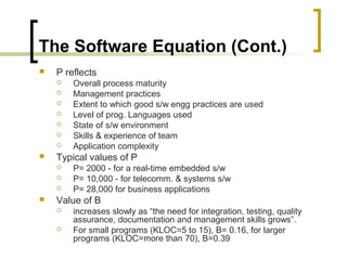
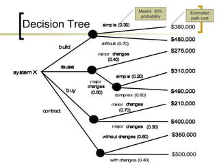
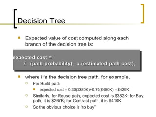
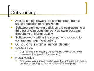
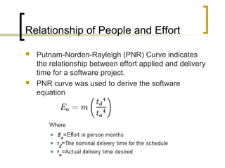
This document provides an outline and summary of topics from lectures on software project management and scheduling. It discusses estimating effort, costs, and resources for a project. Other topics covered include the software equation for estimating effort, make-or-buy decisions, outsourcing, reasons for late delivery, and principles of project scheduling such as interdependencies between tasks. It also describes the relationship between people assigned to a project and effort over time based on the Putnam-Norden-Rayleigh curve.

1. Software Project Management
Lecture # 6

2. Outline
 Recap of topics from Chapter 23
 Remaining topics of Chapter 23
 The Software Equation
 The Make/Buy Decision
 Outsourcing
 Project Scheduling (Chapter 24)
 What is Scheduling?
 What is Tracking?
 Project Scheduling
 Late Software Delivery & Project Deadlines
 Project Scheduling Principles
 People and Effort Relationship

3. Recap – “Software Estimation”
 Software project planner must estimate the following
important things before the project begins
 How long it will take?
 How much effort will be required?
 How much money will be involved?
 How many resources will be required?
 People
 Reusable software
 Software/hardware
 Risk consideration
 In the beginning, project’s scope and feasibility are
determined. The scope helps develop estimates using one
or more techniques that fall into 2 broad categories
 Decomposition
 Empirical modeling

4. Recap – “Software Estimation”
 Decomposition involves identifying major software
function followed by estimates for each
 Empirical techniques use empirically derived
expressions for effort and time estimation
 Software estimation can never be an exact science
but use of good historical data and systematic
techniques can improve estimation accuracy

5. The Software Equation
 Suggested by Putnam & Myers
 It is a multivariable model
 It assumes a specific distribution of effort over life of
s/w project
 It has been derived from productivity data collected
for over 4000 modern-day s/w projects
 E = [LOC x B0.333
/ P]3
x (1/t4
)
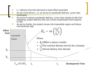
 E = effort in person-months or person-years
 B = special skills factor
 P = productivity factor
 t = project duration (months or years)

6. The Software Equation (Cont.)
 P reflects
 Overall process maturity
 Management practices
 Extent to which good s/w engg practices are used
 Level of prog. Languages used
 State of s/w environment
 Skills & experience of team
 Application complexity
 Typical values of P
 P= 2000 - for a real-time embedded s/w
 P= 10,000 - for telecomm. & systems s/w
 P= 28,000 for business applications
 Value of B
 increases slowly as “the need for integration, testing, quality
assurance, documentation and management skills grows”.
 For small programs (KLOC=5 to 15), B= 0.16, for larger
programs (KLOC=more than 70), B=0.39

7. The Software Equation (Cont.)
 Software equation has two independent parameters
 LOC
 t
 Minimum dev. Time equations derived from
software equation
 tmin= 8.14 (LOC/P)0.43
 in months for tmin> 6 months
 E = 180 Bt3
 In person-months for E>= 20 person-months

8. The Make/Buy decision
 Often it is more cost effective to acquire rather than
develop a software
 Software managers have following options while
making make/buy decisions
 Software may be purchased (or licensed) off the shelf
 “Full experience” or “partial experience” software
components may be acquired and then modified as
needed
 Software may be custom-built by an outside contractor to
meet specifications
 Software criticality to be purchased and the end
cost also affect acquisition process

9. The Make/Buy decision (Cont.)
 For each of the discussed acquisition
options, the Make/Buy decision is made
based on following conditions
 Will he software product be available sooner
than internally developed software?
 Will the acquisition cost plus cost of
customization be less than cost of developing
the software internally?
 Will the cost of outside support (e.g.,
maintenance contract) be less than the cost of
internal support?

10. Decision Tree
system Xsystem X
reusereuse
simple (0.30)simple (0.30)
difficult (0.70)difficult (0.70)
minorminor changeschanges
(0.40)(0.40)
majormajor
changeschanges
(0.60)(0.60)
simple (0.20)simple (0.20)
complex (0.80)complex (0.80)
majormajor changeschanges (0.30)(0.30)
minorminor changeschanges
(0.70)(0.70)
$380,000$380,000
$450,000$450,000
$275,000$275,000
$310,000$310,000
$490,000$490,000
$210,000$210,000
$400,000$400,000
buybuy
contractcontract
without changes (0.60)without changes (0.60)
with changes (0.40)with changes (0.40)
$350,000$350,000
$500,000$500,000
buildbuild
Estimated
path cost
Means 30%
probability

11.  Expected value of cost computed along each
branch of the decision tree is:
 where i is the decision tree path, for example,
 For Build path
 expected cost = 0.30($380K)+0.70($450K) = $429K
 Similarly, for Reuse path, expected cost is $382K; for Buy
path, it is $267K; for Contract path, it is $410K.
 So the obvious choice is “to buy”
Decision Tree
ΣΣ (path probability)(path probability)ii x (estimated path cost)x (estimated path cost)ii
expected cost =expected cost =

12. Outsourcing
 Acquisition of software (or components) from a
source outside the organization
 Software engineering activities are contracted to a
third party who does the work at lower cost and
(hopefully) at higher quality
 Software work within the company is reduced to
contract management activity
 Outsourcing is often a financial decision
 Positive side
 Cost saving can usually be achieved by reducing own
resources (people & infrastructure)
 Negative side
 Company loses some control over the software and bears
the risk of putting its fate in hands of a third party

13. Project Scheduling (Chap. 24 )

14. Introduction
 After the following have been achieved…
 Process model selection
 S/w engg. tasks identification
 Estimation of amount of work & people
 Risk consideration and knowing deadline
 … the task is to create a setup for achieving
the software engineering tasks. This setup is
called ‘software project scheduling and
tracking’

15. What is scheduling?
 An activity that distributes estimated
effort across the planned project
duration by allocating the effort to
specific software engineering task
 Creating a network of software
engineering tasks to complete the
project and assign responsibilities of
tasks and timing of tasks

16. What is Tracking?
 Tracking is the process to make sure
that all tasks are completed according
to assigned responsibility and
schedule.

17. Overview – Proper Scheduling
 Proper Project Scheduling requires
 All tasks should appear in the network
 Interdependencies between tasks are indicated
 Effort and timing are intelligently allocated to
tasks
 Resources are allocated to tasks
 Closely spaced milestones are provided for
progress tracking

18. Reasons for late software delivery
 Unrealistic deadline established by some one
outside the software development group & enforced
 Changing customer requirements that are not
reflected in schedule change
 An honest underestimate of the amount of work
and/or resources required
 Risks that were not considered at project
commencement
 Technical difficulties not foreseen in advance
 Miscommunication among project staff
 A failure by project management to recognize that
the project is falling behind schedule and a lack of
action to correct the problem.

19. Dealing With Project Deadlines
 Aggressive (actually unrealistic) deadlines are a fact
of life in software business
 If best estimates indicate that deadline is unrealistic
Project Manager should
“Protect his/her team from undue (schedule)
pressure… and reflect pressure back to its
originators.”
 Recommended steps for such situations:
1. Perform a detailed estimate using historical data from past
projects. Determine effort and time required.
2. Use incremental model, develop a strategy that will deliver
critical functionality within imposed deadline, but delay
other functionality until later. Document the plan.

20. Dealing With Project Deadlines
3. Meet the customer and explain why deadline is
unrealistic. Explain what is the new time required to
complete this project.
4. Offer incremental development strategy as alternative.
Offer some options.
 We can increase the budget and have bring resources to get
this job done in due time. But this contains increased risk of
poor quality due to tight timeline.
 We can remove some software functions, and provide
remaining functionality later.
 Dispense with reality and wish to complete software in due
time.
 By presenting solid estimates and references to
past projects, it is likely that, negotiated version
option 1 and 2 will be accepted by customer.

21. Project Schedule (Evolution)
 Project schedules evolve over time
 During early stages of project planning, a
macroscopic schedule is developed
 This schedule identifies all major process
framework activities and the product functions to
which they are applied
 As the project proceeds, each entry on the
macroscopic schedule gets refined into detailed
schedule
 Specific tasks are identified to achieve each activity
and are scheduled

22. Project Scheduling - Basic Principles
 Compartmentalization
 Both the product and the process are decomposed into a
number of manageable activities/tasks
 Interdependency
 Interdependencies among decomposed activities must be
identified.
 Some tasks can be performed in sequence and other can
be done in parallel.
 Some activities can not be performed without completion
of another and some can be totally independent
 Time Allocation
 Each task must be allocated work units (person-days of
effort)
 Start and end time must be allocated considering
interdependencies

23. Project Scheduling - Basic Principles
 Effort validation
 Project manager must ensure that no more than the
allocated no. of people have been scheduled at any given
time
 Defined responsibilities
 Every scheduled task must be assigned to a specific team
member
 Defined outcomes
 Work products must be defined for every scheduled task
 Defined milestones
 Every task/group of tasks must be associated with a
project milestone. A milestone is accomplished after one
or more related work products has been reviewed for
quality and approved

24. Relationship of People and Effort
 Common Myth …
 “If we fall behind schedule, we can always add
more programmers and catch up later in the
project!”
 Doing so is often disruptive rather than
productive causing further delays. Reasons:
 learning time
 teaching takes time away from productive work
 added communication paths – increased
complexity

25. Relationship of People and Effort
 Putnam-Norden-Rayleigh (PNR) Curve indicates
the relationship between effort applied and delivery
time for a software project.
 PNR curve was used to derive the software
equation

26.  to = delivery time that will result in least effort expended
 As we move left to to, i.e. as we try to accelerate delivery, curve rises
nonlinearly
 As we try to reduce accelerate delivery, curve rises sharply to left of td
indicating, project delivery time can not be compressed much beyond
0.75td
 As we try further, the project moves into impossible region and failure
risk becomes high
Tmin=0.75Td td to Development Time
Effort
Cost
Ed
Eo
Impossible
Region

27. PNR Curve & Software Eqn.
 The software equation is derived from the PNR
curve
 It demonstrates a highly nonlinear relationship
between time to complete project and human effort
applied to the project
 Lines of Code (L) is related to effort (E) and
development time (t) as:
 L = P x E 1/3
t 4/3
 Rearranging the equation
 E = L3
/ P3
t4