The document defines key concepts in linear kinematics including:
1) Spatial reference frames which provide axes to describe position and direction in 1, 2, or 3 dimensions.
2) Linear concepts such as position, displacement, distance, velocity, and speed. Displacement is the change in position, velocity is the rate of change of position, and speed is the distance traveled per unit time.
3) Methods for calculating displacement, velocity, and speed using change in position over change in time. Velocity is a vector while speed is a scalar.
This document discusses feature extraction and edge detection techniques in computer vision. It provides details on:
1) Edge detection methods including first and second derivative operators, Sobel edge detector, Laplacian of Gaussian (LoG), and Canny edge detector.
2) Edge descriptors such as edge normal, direction, position, and strength.
3) Types of edges like step, ramp, line, and roof edges.
4) Corner detection using an eigenvalue analysis of the gradient matrix within a neighborhood.
Harris corner detector provides rotation invariant feature detection by analyzing the eigenvalues of the Hessian matrix computed at each point. Scale invariant detectors like SIFT find maxima of scale-space functions like the Laplacian of Gaussian or Difference of Gaussians to identify keypoints independently across scale. Affine invariant detectors search for intensity extrema along radial lines from seed points and approximate corresponding image regions with ellipses related by the geometric moment invariants. Descriptors aim to provide distinctive yet invariant representations of local image patches centered on detected keypoints to enable reliable matching across variations.
The Harris corner detector improves upon the Moravec detector. It uses a Gaussian window function instead of a binary one, considers all small shifts using a Taylor expansion, and defines a new corner response measure R based on the eigenvalues of the image derivative matrix M. A point is classified as a corner if R is above a threshold and is a local maximum of R, indicating a large intensity change in all directions at that point.
This document discusses various feature detectors used in computer vision. It begins by describing classic detectors such as the Harris detector and Hessian detector that search scale space to find distinguished locations. It then discusses detecting features at multiple scales using the Laplacian of Gaussian and determinant of Hessian. The document also covers affine covariant detectors such as maximally stable extremal regions and affine shape adaptation. It discusses approaches for speeding up detection using approximations like those in SURF and learning to emulate detectors. Finally, it outlines new developments in feature detection.
This document discusses feature extraction in computer vision systems. It focuses on edge and corner detection methods. Edge detection aims to locate boundaries between objects and background in images. Common approaches discussed include Sobel and Canny edge detectors, which apply first and second derivative filters to detect edges. Corner detection aims to find stable points of interest across images for tracking objects. It involves computing the eigenvalues of a matrix formed from the image gradient to identify corners.
NIPS2008: tutorial: statistical models of visual imageszukun
The document discusses statistical image models and modeling techniques. It describes how photographic images contain diverse specialized structures like edges, textures, and smooth regions that occupy a small region of the full space of all possible images. It advocates using probability models rather than describing images as deterministic manifolds. It outlines different types of density models like nonparametric and parametric/constrained models and the historical trend towards more constrained models.
This document discusses quantifying measurement uncertainty. There are two main sources of uncertainty: a repeatable component and a random component. The random component incorporates all factors affecting measurement precision and leads to uncertainty in measured and calculated values. There are two approaches to quantifying standard uncertainty: Type A uses statistical analysis of replicates, while Type B uses best estimates from other factors like instrument specifications. Standard uncertainty is reported with measured values to indicate the precision of the measurement.
ICASSP2012 Poster Estimating the spin of a table tennis ball using inverse co...Toru Tamaki
Tamaki Toru, Haoming Wang, Bisser Raytchev, Kazufumi Kaneda, Yukihiko Ushiyama: "Estimating the spin of a table tennis ball using inverse compositional image alignment", Proc. of ICASSP 2012 ; 2012 IEEE International Conference on Acoustics, Speech, and Signal Processing,pp. 1457-1460 (2012 03), Kyoto International Conference Center , Kyoto, Japan, March 25-30, 2012.
The document discusses digital filter structures. It covers IIR and FIR filter structures. For IIR filters, it describes direct form I and II structures as well as cascade form using biquad sections. Cascade form implements the IIR filter as a product of second-order filter sections in a direct form structure. FIR filters can be implemented using direct form or cascade of direct form filter sections. The choice of structure depends on factors like complexity, memory requirements, and quantization effects.
The document provides an overview and review of topics related to tracking and filtering fundamentals, including:
- Linear algebra and linear systems, probability, hypothesis testing, and state estimation.
- Linear and non-linear filtering, multiple model filtering, track maintenance, data association techniques, and activity control.
- Mathematics topics like linear algebra, probability, estimation, vector/matrix properties, and state-space representations are reviewed for continuous and discrete time systems. Concepts include the Jacobian, gradient, Dirac delta function, and observability criteria.
- Semi Regular Meshes can be subdivided using regular 1:4 subdivision or represented as Spherical Geometry Images mapped to the unit sphere.
- Subdivision Surfaces are generated by applying local interpolators repeatedly to refine a coarse control mesh. Common subdivision schemes include Linear, Butterfly, and Loop which are demonstrated in examples.
- Biorthogonal Wavelets can be constructed on meshes using a Lifting Scheme to create wavelet coefficients with vanishing moments, allowing for compression of mesh signals. Invariant neighborhoods are used to analyze the refinement of meshes across scales.
This document discusses Fourier processing and covers topics such as continuous and discrete Fourier bases, sampling, 2D Fourier bases, and Fourier approximation. The continuous Fourier basis uses complex exponentials while the discrete Fourier basis uses a finite number of complex exponentials. Sampling and periodization allow transforming between continuous and discrete settings. The 2D Fourier basis is a product of 1D bases. Fourier approximation represents functions as a sum of complex exponentials.
This document provides information on various mathematical topics including:
1. Graphs of polynomial functions in factorized form such as quadratics, cubics, and quartics.
2. Transformations of functions including translations, reflections, dilations, and their effects on graphs.
3. Exponential, logarithmic, and trigonometric functions and their graphs.
4. Relations, functions, and tests to determine if a relation is a function and if a function is one-to-one or many-to-one.
This document provides an overview of a 2004 CVPR tutorial on nonlinear manifolds in computer vision. The tutorial is divided into four parts that cover: (1) motivation for studying nonlinear manifolds and how differential geometry can be useful in vision, (2) tools from differential geometry like manifolds, tangent spaces, and geodesics, (3) statistics on manifolds like distributions and estimation, and (4) algorithms and applications in computer vision like pose estimation, tracking, and optimal linear projections. Nonlinear manifolds are important in computer vision as the underlying spaces in problems involving constraints like objects on circles or matrices with orthogonality constraints are nonlinear. Differential geometry provides a framework for generalizing tools from vector spaces to nonlinear
DISTINGUISH BETWEEN WALSH TRANSFORM AND HAAR TRANSFORMDip transformsNITHIN KALLE PALLY
walsh transform-1D Walsh Transform kernel is given by:
n - 1
g(x, u) = (1/N) ∏ (-1) bi(x) bn-1-i(u)
i = 0
where, N – no. of samples
n – no. of bits needed to represent x as well as u
bk(z) – kth bits in binary representation of z.
Thus, Forward Discrete Walsh Transformation is
N - 1 n - 1
W(u) = (1/N) Σ f(x) ∏ (-1) bi(x) b(u) x = 0 i = 0
The document describes methods for tomographic focusing using polarimetric SAR (PolSAR) data, including:
1) A hybrid spectral approach using CAPON and weighted signal subspace fitting to estimate volume boundaries and ground topography from tropical forest data.
2) A single-baseline PolInSAR technique using an RVOG coherence model to retrieve ground elevation and volume coherence from the data.
3) Experimental results applying these methods to P-band PolSAR data collected over tropical forests in Paracou, France.
Structured regression for efficient object detectionzukun
This document summarizes research on structured regression for efficient object detection. It proposes framing object localization as a structured output regression problem rather than a classification problem. This involves learning a function that maps images directly to object bounding boxes. It describes using a structured support vector machine with joint image/box kernels and box overlap loss to learn this mapping from training data. The document also outlines techniques for efficiently solving the resulting argmax problem using branch-and-bound optimization and discusses extensions to other tasks like image segmentation.
The document discusses slope and how to calculate it. Slope is defined as the ratio of vertical distance change to horizontal distance change between two points on a line. The formula for slope is provided as m=(y2-y1)/(x2-x1). Several examples are worked through to demonstrate calculating slope for different lines by using points on each line in the formula. Horizontal and vertical lines are also discussed, with horizontal lines having a slope of 0 and vertical lines having an undefined slope.
This document provides an introduction to digital image processing. It discusses key topics like image representation as matrices, image digitization which involves sampling and quantization, and the basic steps in digital image processing such as image acquisition, preprocessing, segmentation, feature extraction, recognition and interpretation. Importance of image processing is highlighted for applications like remote sensing, machine vision, and medical imaging. Common techniques like noise filtering, contrast enhancement, compression and their importance are also summarized.
The document outlines research on developing optimal finite difference grids for solving elliptic and parabolic partial differential equations (PDEs). It introduces the motivation to accurately compute Neumann-to-Dirichlet (NtD) maps. It then summarizes the formulation and discretization of model elliptic and parabolic PDE problems, including deriving the discrete NtD map. It presents results on optimal grid design and the spectral accuracy achieved. Future work is proposed on extending the NtD map approach to non-uniformly spaced boundary data.
The document discusses properties and applications of the Z-transform, which is used to analyze linear discrete-time signals. Some key points:
1) The Z-transform plays an important role in analyzing discrete-time signals and is defined as the sum of the signal samples multiplied by a complex variable z raised to the power of the sample's time index.
2) Important properties of the Z-transform include linearity, time-shifting, frequency-shifting, differentiation in the Z-domain, and the convolution theorem.
3) The Z-transform can be used to find the transform of basic sequences like the unit impulse, unit step, exponentials, polynomials, and derivatives of signals.
This document discusses Bayesian nonparametric posterior concentration rates under different loss functions.
1. It provides an overview of posterior concentration, how it gives insights into priors and inference, and how minimax rates can characterize concentration classes.
2. The proof technique involves constructing tests and relating distances like KL divergence to the loss function. Examples where nice results exist include density estimation, regression, and white noise models.
3. For the white noise model with a random truncation prior, it shows L2 concentration and pointwise concentration rates match minimax. But for sup-norm loss, existing results only achieve a suboptimal rate. The document explores how to potentially obtain better adaptation for sup-norm loss.
Stuff You Must Know Cold for the AP Calculus BC Exam!A Jorge Garcia
This document provides a summary of key concepts from AP Calculus that students must know, including:
- Differentiation rules like product rule, quotient rule, and chain rule
- Integration techniques like Riemann sums, trapezoidal rule, and Simpson's rule
- Theorems related to derivatives and integrals like the Mean Value Theorem, Fundamental Theorem of Calculus, and Rolle's Theorem
- Common trigonometric derivatives and integrals
- Series approximations like Taylor series and Maclaurin series
- Calculus topics for polar coordinates, parametric equations, and vectors
The document discusses the definition and properties of a parabola. A parabola is defined as the locus of a point where the distance from a fixed point (the focus) is equal to the distance from a fixed line (the directrix). Key properties include:
- The vertex is at (0,0)
- The equation relating x, y, and the focal length a is x2 = 4ay
- Given this equation, one can find the focus, directrix, and focal length
Using Graph Partitioning Techniques for Neighbour Selection in User-Based Col...Alejandro Bellogin
Using graph partitioning techniques like Normalised Cut (NCut) for neighbourhood selection in user-based collaborative filtering outperforms other clustering methods like k-Means. NCut models users as nodes in a graph and clusters them based on their similarities. It was tested on the Movielens 100K dataset against baselines like user-based CF with Pearson correlation and matrix factorization. NCut achieved higher precision and coverage than the baselines, showing the benefit of using graph partitioning for neighbourhood selection in collaborative filtering.
1) The document discusses machine learning concepts including polynomial curve fitting, probability theory, maximum likelihood, Bayesian approaches, and model selection.
2) It describes using polynomial functions to fit a curve to data points and minimizing the error between predictions and actual target values. Higher order polynomials can overfit noise in the data.
3) Regularization is introduced to add a penalty for high coefficient values in complex models to reduce overfitting, analogous to limiting the polynomial order. This improves generalization to new data.
Rapoart de cercetare științifică nr.2
Modele biomecanice propuse pentru studiul aparatului locomotor uman sub acțiunea vibrațiilor.
Cuprinsul raportului 2 ( prezentarea are 45 de slideuri) ,, Capitolul 1 (2 slide-uri), Introducere,1.1. Domeniul de studiu, 1.2. Scop și obiectiv 1.3. Principiile modelării Capitolul 2. (11 slide-uri) Biocinematica. 2.1. Sisteme de referință 2.2. Transformări omogene 2.3 Convenția DENAVITT-HARTENBERG, Capitolul 3 (7 slide-uri) Modelul cinematic 3.1. Cazul general 3.2. Modelarea cinematică a membrului inferior, Capitolul 4 (7 slide-uri) Modelarea solicitărilor statice şi dinamice ale sistemelor anatomice gleznă-picior şi genunchi – gambă, Capitolul 5 (4 slide-uri), Expunerea organismului uman la vibrații, Capitolul 6 (5 slide-uri), Studiul stabilității unei proteze de gambă cu ajutorul mediului simulink. Și Ultimul capitol. Capitolul 7 (5 slide-uri)Model biomecanic al gleznei realizat în Simmechanics.
(lucrarea se încheie cu Bibliografie).
This document discusses fundamental concepts in analytic geometry related to lines. It defines key terms like slope, the different forms of a line equation, and how to find the distance from a point to a line. It also covers properties and elements of triangles, including how to calculate the length of a median, altitude, and angle bisector.
The document provides an overview of different techniques for scan conversion of points, lines, and circles. It discusses point plotting, random scan conversion, and raster scan conversion of points. For lines, it describes direct use of the line equation, the Digital Differential Analyzer (DDA) algorithm, and Bresenham's line algorithm. Bresenham's algorithm uses only incremental integer calculations to accurately and efficiently determine pixel positions along a line path.
This document discusses 2D geometric transformations including translation, rotation, scaling, and composite transformations. It provides definitions and formulas for each type of transformation. Translation moves objects by adding offsets to coordinates without deformation. Rotation rotates objects around an origin by a certain angle. Scaling enlarges or shrinks objects by multiplying coordinates by scaling factors. Composite transformations apply multiple transformations sequentially by multiplying their matrices. Homogeneous coordinates are also introduced to represent transformations in matrix form.
Two-dimensional transformations include translations, rotations, and scalings. Transformations manipulate objects by altering their coordinate descriptions without redrawing them. Matrices can represent linear transformations and are used to describe 2D transformations. Common 2D transformations include translation by adding offsets to coordinates, rotation by applying a rotation matrix, and scaling by multiplying coordinates by scaling factors. More complex transformations can be achieved by combining basic transformations through matrix multiplication in a specific order.
This chapter discusses key concepts related to straight lines including:
1) Gradient represents the steepness of a line and is calculated by the rise over run between two points;
2) Gradient can be positive, negative, or undefined based on the line's direction;
3) The equation of a straight line can be written in slope-intercept or point-slope form using the gradient and a point;
4) Lines are parallel if they have the same gradient.
This document provides definitions and notations for 2-D systems and matrices. It defines how continuous and sampled 2-D signals like images are represented. It introduces some common 2-D functions used in signal processing like the Dirac delta, rectangle, and sinc functions. It describes how 2-D linear systems can be represented by matrices and discusses properties of the 2-D Fourier transform including the frequency response and eigenfunctions. It also introduces concepts of Toeplitz and circulant matrices and provides an example of convolving periodic sequences using circulant matrices. Finally, it defines orthogonal and unitary matrices.
This document discusses various mathematical tools used in digital image processing (DIP), including array versus matrix operations, linear versus nonlinear operations, arithmetic operations, set and logical operations, spatial operations, vector and matrix operations, and image transforms. Key points include:
- Array operations are performed on a pixel-by-pixel basis, while matrix operations consider relationships between pixels.
- Linear operators preserve scaling and addition properties, while nonlinear operators like max do not.
- Spatial operations include single-pixel, neighborhood, and geometric transformations of pixel locations and intensities.
- Images can be represented as vectors and transformed using matrix operations.
- Common transforms like Fourier use separable, symmetric kernels to decompose images into frequency domains.
Here are the steps to solve these problems:
1. Find the slopes of the two lines:
m1 = (8-2)/(5--2) = 6/3 = 2 (slope of r)
m2 = (7-0)/(-8--2) = 7/-6 = -1 (slope of s)
The slopes are negative reciprocals, so r ⊥ s.
2. The slopes are m1 = 2 and m2 = -1/2. Since m1 × m2 = -1, the lines are perpendicular.
3. The given line has slope 3. The perpendicular line will have slope -1/3. Plug into the point-slope form
Geometric transformations play an important role in computer graphics by allowing graphics to be repositioned on the screen or changed in size and orientation. There are several types of 2D transformations including translation, rotation, scaling, reflection, and shearing. Translation moves an object by translating each vertex by a certain distance. Rotation moves a point around a center point by a certain angle. Scaling enlarges or shrinks an object by a scaling factor. Reflection produces a mirror image of an object across an axis. Shearing distorts an object by shifting coordinate values.
This document discusses 2D and 3D transformations. It begins with an overview of basic 2D transformations like translation, scaling, rotation, and shearing. It then covers representing transformations with matrices and combining transformations through matrix multiplication. Homogeneous coordinates are introduced as a way to represent translations with matrices. The key transformations can all be represented as 3x3 matrices using homogeneous coordinates.
The document describes algorithms for scan converting primitive geometric objects like lines, circles, and ellipses. It explains Bresenham's line algorithm which uses integer arithmetic to efficiently determine the pixel locations along a line path, getting closer to the actual line than the traditional Digital Differential Analyzer (DDA) algorithm. It also covers the midpoint circle algorithm which uses distance comparison to test the midpoint between pixels to decide if it is inside or outside the circle boundary during scan conversion.
This document discusses 2D transformations including translation, rotation, scaling, shearing, and reflection. It explains how to represent points in 2D using vectors and matrices. Various transformation matrices are defined to transform points and geometries through translation, rotation about a pivot point, uniform and non-uniform scaling, reflection across lines or planes, and shearing. Composite transformations consisting of multiple simple transformations applied sequentially are also discussed. Examples are provided to demonstrate how common geometries like lines and polygons are transformed.
The document discusses slopes and equations of lines. It defines slope as rise over run and provides formulas for calculating slope given two points on a line. It explains that the slope-intercept form is y=mx+b and point-slope form is y-y1=m(x-x1). Examples are given of writing equations of lines given slope and a point or y-intercept. Horizontal and vertical lines are also addressed.
1) 2-D geometric transformations allow manipulation of objects in 2-D space by changing their position, size, and orientation.
2) The basic geometric transformations are translation, rotation, scaling, reflection, and shear. Translation moves an object by shifting its coordinates. Rotation turns an object around a fixed point. Scaling enlarges or shrinks an object. Reflection produces a mirror image. Shear distorts an object.
3) Each transformation can be described by a matrix equation. The inverse of a transformation performs the opposite operation to return the object to its original state.
This document discusses various two-dimensional geometric transformations including translations, rotations, scaling, reflections, shears, and composite transformations. Translations move objects without deformation using a translation vector. Rotations rotate objects around a fixed point or pivot point. Scaling transformations enlarge or shrink objects using scaling factors. Reflections produce a mirror image of an object across an axis. Shearing slants an object along an axis. Composite transformations combine multiple basic transformations using matrix multiplication.
The document provides information about linear equations and their graphs. It defines linear equations and discusses how to write equations in slope-intercept form, point-slope form, and standard form. It also describes how to graph linear equations by plotting intercepts and using slope. Key topics covered include finding the slope between two points, determining if lines are parallel or perpendicular based on their slopes, and recognizing the intercepts on a graph of a linear equation in two variables.
Digital signatures are often used to implement electronic signatures, a broader term that refers to any electronic data that carries the intent of a signature, but not all electronic signatures use digital signatures. In some countries, including the United States, India, and members of the European Union, electronic signatures have legal significance.
The document discusses various techniques for image segmentation including discontinuity-based approaches, similarity-based approaches, thresholding methods, region-based segmentation using region growing and region splitting/merging. Key techniques covered include edge detection using gradient operators, the Hough transform for edge linking, optimal thresholding, and split-and-merge segmentation using quadtrees.
Parametric equations describe curves using two functions, one for the x-coordinates and one for the y-coordinates, rather than a single function relating x and y. They allow curves to be described that cannot be expressed as a single-valued function. The parameter, often representing time or an angle, does not appear in the final graph but is used to generate the coordinates.
Theo measured an angle of 0.6 degrees between the base and top of a building when standing 4000 feet from the base. To calculate the height of the building, the document explains different forms of writing linear equations, including general, slope-intercept, double-intercept, point-slope, and two-point forms. It then provides examples of writing equations in these different forms and converting between forms.
The document provides a math review covering topics in algebra, geometry, trigonometry, and statistics. It defines concepts like negative numbers, exponents, square roots, order of operations, lines, angles, trigonometric functions, and averages. Formulas are presented for topics like quadratic equations, the Pythagorean theorem, laws of sines and cosines, percentages, and standard deviation. Examples are included to illustrate key ideas.
The document provides an overview of solving biomechanics problems, distinguishing between qualitative and quantitative approaches. It discusses solving formal quantitative problems through a step-by-step process of understanding the problem, identifying known and unknown values, selecting applicable formulas, performing calculations, and checking results. Examples of quantitative problems are provided along with discussions of units, conversions, and evaluating whether answers are reasonable.
1) The document defines three types of motion - translation, angular, and general - and describes anatomical reference positions, planes, axes, and directional terms used to qualitatively analyze human movement.
2) It provides details on planar movements including flexion/extension, abduction/adduction, and internal/external rotation in the sagittal, frontal, and transverse planes respectively.
3) Qualitative analysis of human movement involves descriptive observation of technique and performance to identify causes of problems and differentiate unrelated factors, and the document outlines steps to plan and conduct such an analysis.
The document defines vectors and describes various vector operations that can be performed, including:
- Graphical vector addition using the tip-to-tail method
- Numerical representation of vectors using magnitude, direction, and components
- Resolution of a vector into perpendicular components
- Composition and decomposition of vectors using graphical and numerical methods
- Scalar multiplication and subtraction of vectors
It also provides examples of how to use vectors to solve problems graphically or numerically.
This document introduces the concepts of linear acceleration, computing acceleration from changes in velocity over time, and the differences between average and instantaneous acceleration. It provides examples of calculating acceleration from velocity data and graphs, and reviews the laws of constant acceleration for relating changes in velocity, displacement, and time when acceleration is constant. Key topics covered include computing acceleration from changes in velocity and time, using graphs of velocity over time to determine acceleration, and applying the kinematic equations for constant acceleration.
The document discusses projectile motion, which describes the trajectory of objects in free fall under only the forces of gravity and air resistance. It defines a projectile and explains how gravity influences the vertical and horizontal components of motion differently. Key factors that determine a projectile's trajectory include the projection angle, speed, and height. Optimal projection conditions exist that maximize distance or height based on these factors. Examples are provided to demonstrate how to calculate values like maximum height, flight time, and distance for a given projectile scenario.
1) Angular kinematics describes motion that involves rotation, such as the movement of body segments. It includes concepts like angular displacement, velocity, and speed.
2) Key concepts in angular kinematics include computing angular quantities from changes in angular position over time, using degrees and radians as units of angle, and determining average versus instantaneous angular velocity.
3) Joint angles are relative angles between adjacent body segments and are important for analyzing human movement.
Angular acceleration is the rate of change of angular velocity over time. It is calculated as the change in angular velocity divided by the change in time. Angular acceleration, like linear acceleration, can be constant or varying. For constant angular acceleration, the angular kinematic equations relating angular displacement, velocity, acceleration, and time can be used. Understanding the relationships between linear and angular quantities like distance, speed, and acceleration is important when analyzing rotational or spinning motion.
This document discusses linear and angular motion concepts including:
1) The relationship between linear and angular velocity for rotating bodies
2) Computing tangental and radial acceleration of rotating bodies
3) Analyzing general motion involving combinations of linear and angular movement
4) Methods for measuring kinematic quantities such as velocity and acceleration.
Kinetics is the study of the relationship between forces acting on a system and its motion. It includes concepts like inertia, mass, force, weight, torque, and impulse. Forces can cause both acceleration and deformation of objects. Stress is the force distributed over an area, while pressure is the stress due to compression. Materials respond elastically to small loads but experience permanent plastic deformation above the yield point, with rupture occurring at ultimate failure. Repeated cyclic loading reduces the stress needed to cause material failure compared to a single acute load.
This document defines linear kinetics and describes Newton's three laws of motion. Linear kinetics is the study of the relationship between forces and motion for objects undergoing linear or translational motion. Newton's first law states that an object at rest stays at rest or an object in motion stays in motion with constant velocity unless acted upon by an external force. The second law relates the external force on an object to its mass and acceleration. The third law states that for every action force there is an equal and opposite reaction force. Examples are also given to illustrate applications of the laws.
1) Momentum is defined as the product of an object's mass and velocity. It is a vector quantity that represents the quantity of motion.
2) The principle of conservation of momentum states that if the total external force on a system is zero, the total momentum of the system remains constant.
3) Impulse is defined as the change in momentum of an object due to an applied force over time. According to the impulse-momentum theorem, the impulse applied to an object equals its change in momentum.
Mechanical work is the product of the force applied and the displacement in the direction of the force. Power is the rate of work done over time. There are two types of energy: kinetic energy, which is the energy of motion, and potential energy, which is stored energy due to an object's position or deformation. The total energy of an isolated system remains constant according to the principle of conservation of energy. Friction is a force that opposes motion between two surfaces in contact. There are two types of friction: static and kinetic friction.
1) Angular kinetics is the study of forces that cause rotation or torques. Torque is a measure of how much a force causes an object to rotate and depends on the force magnitude and its moment arm.
2) The moment arm is the distance from the axis of rotation to where the force is applied. Torque is calculated by multiplying the force by the moment arm.
3) Resultant joint torque is the single torque that has the same rotational effect as all the individual torques acting on a joint. It provides a simplified view of which muscle groups are most active at a joint.
1) Linear and angular kinetics relate external forces/torques to inertia, displacement/angular displacement, velocity/angular velocity, and acceleration/angular acceleration respectively.
2) Moment of inertia represents an object's resistance to changes in angular motion and depends on the object's mass distribution and the axis of rotation.
3) Angular momentum is the product of an object's moment of inertia and angular velocity, and is conserved if no external torque is applied to the system.
The document discusses internal and external torques, the three laws of angular motion, and key concepts related to rotational dynamics including:
1) Internal torque is applied within a system while external torque is applied across the system boundary.
2) The three laws of angular motion describe how torques cause changes in angular velocity and acceleration according to an object's moment of inertia.
3) Key concepts like angular impulse, work, power, and kinetic energy can be analyzed similarly to linear motion but involve torque, angular velocity/acceleration, and moment of inertia rather than force and linear velocity/acceleration.
1) A free body diagram is used to represent all external forces and torques acting on a system. It is an important step in solving kinetics problems.
2) The document provides guidance on constructing free body diagrams including identifying the system, drawing external forces and torques, and specifying the point of application and direction.
3) Lever systems use an effort force to move a load force. There are three classes of levers that vary based on the relative positions of the effort, load, and fulcrum. Mechanical advantage determines the trade off between force and distance of movement.
Stability and balance refer to an object's ability to resist changes to its equilibrium state and return to its original position if disturbed. Key factors that influence stability include an object's mass/moment of inertia, its base of support, the position of its center of mass relative to the base of support, and surface friction. Static balance requires keeping the center of mass over the base of support, while dynamic balance involves controlling the center of mass during movements to prevent losing equilibrium and falling.
- A system is at static equilibrium when it is at rest and experiences no translation or rotation (according to Newton's 1st law). The net external forces and torques on the system must equal zero.
- Dynamic equilibrium applies to accelerating rigid bodies (according to Newton's 2nd law). The net external forces must equal mass times acceleration, and net torque must equal moment of inertia times angular acceleration.
- Inverse dynamics uses measured joint positions, ground reaction forces, and segment parameters to compute unknown joint forces and torques that produce the observed motion. Segments are analyzed individually from distal to proximal.
Biomechanics is the application of mechanical principles to the study of living organisms like the human body. It has two main sub-branches - statics which looks at systems at rest or in constant motion, and dynamics which examines accelerated systems. Biomechanics is used by professionals in sports, health, rehabilitation and engineering to improve performance, prevent and treat injuries, reduce physical declines, improve mobility, and aid product design. The goal of this introduction is to define key biomechanics concepts and illustrate its wide-ranging applications.
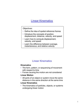
1. Linear Kinematics
Objectives:
• Define the idea of spatial reference frames
• Introduce the concepts of position,
displacement, distance, velocity, and speed
• Learn how to compute displacement,
velocity, and speed
• Learn the difference between average,
instantaneous, and relative velocity
Linear Kinematics
Kinematics
• The form, pattern, or sequencing of movement
with respect to time
• Forces causing the motion are not considered
Linear Motion
• All parts of an object or system move the same
distance in the same direction at the same time
Linear Kinematics
• The kinematics of particles, objects, or systems
undergoing linear motion
1
2. Spatial Reference Frames
• A spatial reference frame is a set of coordinate axes
(1, 2, or 3), oriented perpendicular to each other.
• It provides a means of describing and quantifying
positions and directions in space
1-dimensional (1-D) Reference Frame
• Quantifies positions and directions along a line
unit of measure
origin
label
x = 2m
x (m)
-5 -4 -3 -2 -1 0 1 2 3 4 5
– direction + direction
2-D Reference Frame
• Quantifies positions and directions in a plane
y (m)
(x,y) = (1 m, 2 m)
2
+y direction
–y direction
unit of measure
label
90° θ=63°
(0,0) x (m)
-2 2
origin +x direction
–x direction
2
3. 3-D Reference Frame
• Quantifies positions and directions in space
z (m)
2
(x,y,z) = (1.5m, 2m, 1.8m)
(0,0,0)
φ=36°
y (m)
2
θ=53°
x (m) 2
Reference Frames & Motion
• The position or motion of a system does not
depend on the choice of reference frame
• But, the numbers used to describe them do
• Always specify the reference frame used!
y1 (m)
)
(m
x2
)
(m
y2
1
1
1
x1 (m)
1
3
4. Selecting a Reference Frame
• Use only as many dimensions as necessary
• Align reference frame with fixed, clearly-defined,
and physically meaningful directions.
(e.g. compass directions, anatomical planes)
Common 2-D conventions:
– Sagittal plane: +X = anterior; +Y = upward
– Transverse plane: +X = left; +Y = upward
– Horizontal plane: +X = anterior; +Y = left
• The origin should also have physical meaning.
2-D examples:
– X=0 initial position
– Y=0 ground height
Position
• The location of a point, with respect to the origin,
within a spatial reference frame
• Position is a vector; has magnitude and direction
• Or, specify position by the coordinates of the point
• Position has units of length (e.g. meters, feet)
y (m) (x,y) = (1m, 2m)
2
Point’s position is:
• distance of 2.24m at an angle
2.24m of 63° above the +x axis, or
• (x,y) position of (1m, 2 m)
origin
θ=63°
x (m)
(0,0) 2
4
5. Linear Displacement
• Change (directed distance) from a point’s initial
position to its final position
• Displacement is a vector; has magnitude and direction
• Displacement has units of length (e.g. meters, feet)
y (m)
initial position
displacement
1 pinitial final position
pfinal
x (m)
1
Computing Displacement
• Compute displacement (∆p) by vector subtraction
∆p = pfinal – pinitial
y (m) initial position
1
pinitial final position
pfinal
x (m)
1
–pinitial –pinitial
∆p
5
6. Describing Displacement
• Can describe displacement by:
– Magnitude and direction
(e.g. 2.23m at 26.6° below the +x axis)
– Components y (m)
(change) along
each axis 1 pinitial
(e.g. 2m in the +x
pfinal
direction, 1m in
1
the –y direction)
θ ∆px x (m)
∆py
∆p
-1
Distance
• The length of the path traveled between a point’s
initial and final position
• Distance is a scalar; it has magnitude only
• Has units of length (e.g. meters, feet)
• Distance ≥ (Magnitude of displacement)
Displacement
= 64 m West
E
N
Distance = 200m
6
7. Example Problem #1
A box is resting on a table of height 0.3m.
A worker lifts the box straight upward to a
height of 1m.
He carries the box straight backward 0.5m,
keeping it at a constant height.
He then lowers the box straight downward to
the ground.
What was the displacement of the box?
What distance was the box moved?
Linear Velocity
• The rate of change of position
• Velocity is a vector; has magnitude and direction
change in position displacement
velocity = =
change in time change in time
• Shorthand notation:
pfinal – pinitial ∆p
v = =
tfinal – tinitial ∆t
• Velocity has units of length/time (e.g. m/s, ft/s)
7
8. Computing Velocity
• direction of velocity = direction of displacement
• magnitude of velocity = magnitude of displacement
change in time
• component of velocity = component of displacement
change in time
y ∆p y V = ∆p / ∆t
t
/∆
∆p
∆p
∆py vy = ∆py / ∆t
=
θ v θ
x x
∆px vx = ∆px / ∆t
Speed
• The distance traveled divided by the time taken
to cover it
• Equal to the average magnitude of the
instantaneous velocity over that time.
distance
speed =
change in time
• Speed is a scalar; has magnitude only
• Speed has units of length/time (e.g. m/s, ft/s)
8
9. Speed vs. Velocity
Displacement
= 64 m West
E
N
Distance = 200m
Assume a runner takes 25 s to run 200 m:
200 m 64 m West
Speed = Velocity =
25 s 25 s
= 8 m/s = 2.6 m/s West
Example Problem #2
During the lifting task of example problem #1, it
takes the worker 0.5s to lift the box, 1.3s to
carry it backward, and 0.6s to lower it.
What were the average velocity and average
speed of the box during the first, lifting phase
of the task?
What were the average velocity and average
speed of the box for the task as a whole?
9
10. Velocity as a Slope
• Graph x-component of position vs. time
• x-component of velocity from t1 to t2
= slope of the line from px at t1 to px at t2
Slope : ∆px / ∆t = vx
px (m)
∆px
∆t
t1 t2 time (s)
Average vs. Instantaneous Velocity
• The previous formulas give us the average velocity
between an initial time (t1) and a final time (t2)
• Instantaneous velocity is the velocity at a single
instant in time
• Can estimate instantaneous velocity using the
central difference method:
p (at t1 + ∆t) – p (at t1 – ∆t)
v (at t1) =
2 ∆t
where ∆t is a very small change in time
10
11. Instantaneous Velocity as a Slope
• Graph of x-component of position vs. time
slope = instantaneous
x-velocity at t1
px (m)
slope = average
x-velocity from
t1 to t2
∆t
t1 t2 time (s)
Estimating Velocity from Position
Identify points with
px (m)
zero slope = points
with zero velocity
Portions of the curve
with positive slope
time (s) have positive velocity
(i.e. velocity in the
vx (m/s)
+ direction)
Portions of the curve
with negative slope
0
time (s) have negative velocity
(i.e. velocity in the
– direction)
11
12. Relative Position
• Find the position of one point or object relative to
another by vector subtraction of their positions
p(2 relative to 1) = p2 – p1
p2 = p1 + p(2 relative to 1)
y (m)
object 2
1 p(2 relative to 1)
p2 object 1
p1
x (m)
1
Relative Velocity
• Apparent velocity of a second point or object to
an observer at a first moving point or object
• Compute by vector subtraction of the velocities
v(2 relative to 1) = v2 – v1
vy (m/s)
v2 = v1 + v(2 relative to 1)
object 2
1 v(2 relative to 1)
v2 object 1
v1
vx (m/s)
1
12
13. Example Problem #3
A runner on a treadmill is running at 3.4 m/s in
a direction 10° left of forward, relative to the
treadmill belt (resulting in a forward velocity
of 3.3 m/s and a leftward velocity of 0.6 m/s,
relative to the belt).
The treadmill belt is moving backward at 3.6
m/s.
What is the runner’s overall velocity?
13