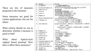
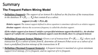
Association rule mining aims to discover interesting relationships between items in large datasets. The document discusses key concepts in association rule mining including support, confidence, and correlation. Support measures how frequently an itemset occurs, while confidence measures the conditional probability of an itemset given another itemset. Correlation evaluates statistical dependence between itemsets and can be used to measure lift. Various measures are proposed to evaluate interestingness and redundancy of discovered rules.

1. Association Analysis to
Correlation Analysis

2. Pattern Evaluation
• Association rule algorithms tend to produce too many rules
‒ many of them are uninteresting or redundant
‒ Redundant if {A,B,C}  {D} and {A,B}  {D} have same
support & confidence
• Interestingness measures can be used to prune/rank the derived
patterns
• In the original formulation of association rules, support & confidence
are the only measures used

3. • Application of Interestingness Measure

4. • Given a rule X  Y, information needed to compute rule interestingness
can be obtained from a contingency table
Y Y
X f11 f10 f1+
X f01 f00 fo+
f+1 f+0 |T|
Contingency table for X  Y
f11: support of X and Y
f10: support of X and Y
f01: support of X and Y
f00: support of X and Y
Used to define various measures
 support, confidence, lift, Gini,
J-measure, etc.
• Computing Interestingness Measure

5. • Drawback of Confidence
Coffee Coffee
Tea 15 5 20
Tea 75 5 80
90 10 100
Association Rule: Tea  Coffee
Confidence= P(Coffee|Tea) = 0.75
but P(Coffee) = 0.9
 Although confidence is high, rule is misleading
 P(Coffee|Tea) = 0.9375

6. Correlation Concepts
• Two item sets A and B are independent (the occurrence of A is
independent of the occurrence of item set B) iff
P(A  B) = P(A)  P(B)
• Otherwise A and B are dependent and correlated
• The measure of correlation, or correlation between A and B is
given by the formula:
Corr(A,B)= P(A U B ) / P(A) . P(B)
6

7. Correlation Concepts [Cont.]
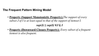
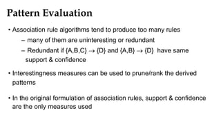
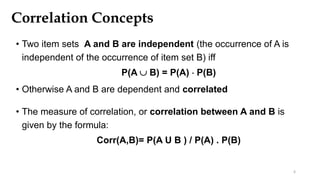
• corr(A,B) >1 means that A and B are positively correlated
i.e. the occurrence of one implies the occurrence of the other.
• corr(A,B) < 1 means that the occurrence of A is negatively correlated
with (or discourages) the occurrence of B.
• corr(A,B) =1 means that A and B are independent and there is no
correlation between them.
7

8. • Statistical Independence
• Population of 1000 students
• 600 students know how to swim (S)
• 700 students know how to bike (B)
• 420 students know how to swim and bike (S,B)
• P(SB) = 420/1000 = 0.42
• P(S)  P(B) = 0.6  0.7 = 0.42
• P(SB) = P(S)  P(B) => Statistical independence
• P(SB) > P(S)  P(B) => Positively correlated
• P(SB) < P(S)  P(B) => Negatively correlated

9. Association & Correlation
• The correlation formula can be re-written as
Corr(A,B) = P(B|A) / P(B)
• We already know that
• Support(A B)= P(AUB)
• Confidence(A  B)= P(B|A)
• That means that, Confidence(A B)= corr(A,B) P(B)
• So correlation, support and confidence are all different, but the correlation
provides an extra information about the association rule (A B).
• We say that the correlation
corr(A,B) provides the LIFT of the association rule (A=>B),
• i.e. A is said to increase (or LIFT) the likelihood of B by the factor of the
value returned by the formula for corr(A,B). 9

10. Statistical-based Measures
• Measures that take into account statistical dependence
)](1)[()](1)[(
)()(),(
)()(),(
)()(
),(
)(
)|(
YPYPXPXP
YPXPYXP
tcoefficien
YPXPYXPPS
YPXP
YXP
Interest
YP
XYP
Lift







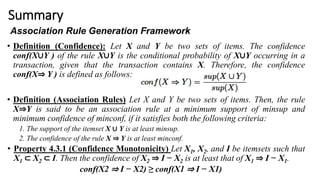
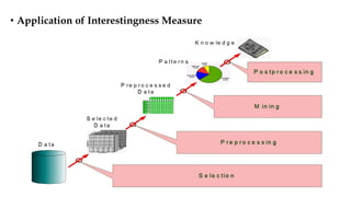
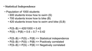
P(A and B) = P(A) x P(B|A)
P(A) x P(B|A) = P(A and B)
P(B|A) = P(A and B) / P(A)

11. Interestingness Measure: Correlations (Lift)
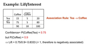
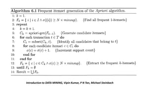
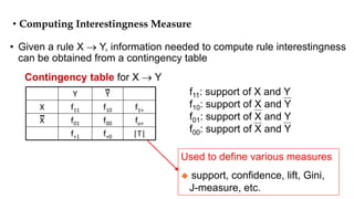
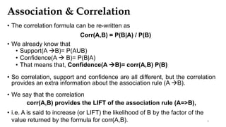
• play basketball  eat cereal [40%, 66.7%] is misleading
• The overall % of students eating cereal is 75% > 66.7%.
• play basketball  not eat cereal [20%, 33.3%] is more accurate, although with lower
support and confidence
• Measure of dependent/correlated events: lift
89.0
5000/3750*5000/3000
5000/2000
),( CBlift
Basketball Not
basketball
Sum
(row)
Cereal 2000 1750 3750
Not cereal 1000 250 1250
Sum(col.) 3000 2000 5000
)()(
)(
BPAP
BAP
lift


33.1
5000/1250*5000/3000
5000/1000
),( CBlift

12. Example: Lift/Interest
Coffee Coffee
Tea 15 5 20
Tea 75 5 80
90 10 100
Confidence= P(Coffee|Tea) = 0.75
but P(Coffee) = 0.9
 Lift = 0.75/0.9= 0.8333 (< 1, therefore is negatively associated)
Association Rule: Tea  Coffee

13. Example: -Coefficient
• -coefficient is analogous to correlation coefficient for continuous
variables
Y Y
X 60 10 70
X 10 20 30
70 30 100
Y Y
X 20 10 30
X 10 60 70
30 70 100
5238.0
3.07.03.07.0
7.07.06.0




 Coefficient is the same for both tables
5238.0
3.07.03.07.0
3.03.02.0





14. There are lots of measures
proposed in the literature
Some measures are good for
certain applications, but not for
others
What criteria should we use to
determine whether a measure is
good or bad?
What about Apriori-style
support based pruning? How
does it affect these measures?

15. Summary
• Definition (Support): The support of an itemset I is defined as the fraction of the transactions
in the database T = {T1 . . . Tn} that contain I as a subset.
support (AB) = P(AB)
Relative support: The itemset support defined in above equation is sometimes referred to as relative support.
Absolute support: whereas the occurrence frequency is called the absolute support.
(If the relative support of an itemset I satisfies a prespecified minimum support threshold (i.e., the absolute
support of I satisfies the corresponding minimum support count threshold), then I is a frequent itemset)
• Definition (Frequent Itemset Mining): Given a set of transactions T = {T1 . . . Tn}, where each
transaction Ti is a subset of items from U, determine all itemsets I that occur as a subset of at
least a predefined fraction minsup of the transactions in T.
• Definition (Maximal Frequent Itemsets): A frequent itemset is maximal at a given minimum
support level minsup, if it is frequent, and no superset of it is frequent.
The Frequent Pattern Mining Model

16. • Property (Support Monotonicity Property):The support of every
subset J of I is at least equal to that of the support of itemset I.
sup(J) ≥ sup(I) ∀J ⊆ I
• Property (Downward Closure Property): Every subset of a frequent
itemset is also frequent.
The Frequent Pattern Mining Model

17. Summary
• Definition (Confidence): Let X and Y be two sets of items. The confidence
conf(X∪Y ) of the rule X∪Y is the conditional probability of X∪Y occurring in a
transaction, given that the transaction contains X. Therefore, the confidence
conf(X⇒ Y ) is defined as follows:
• Definition (Association Rules) Let X and Y be two sets of items. Then, the rule
X⇒Y is said to be an association rule at a minimum support of minsup and
minimum confidence of minconf, if it satisfies both the following criteria:
1. The support of the itemset X ∪ Y is at least minsup.
2. The confidence of the rule X ⇒ Y is at least minconf.
• Property 4.3.1 (Confidence Monotonicity) Let X1, X2, and I be itemsets such that
X1 ⊂ X2 ⊂ I. Then the confidence of X2 ⇒ I − X2 is at least that of X1 ⇒ I − X1.
conf(X2 ⇒ I − X2) ≥ conf(X1 ⇒ I − X1)
Association Rule Generation Framework

18. Introduction to DATA MINING, Vipin Kumar, P N Tan, Michael Steinbach