Download to read offline


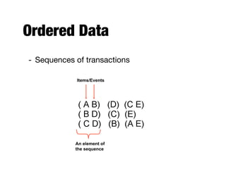

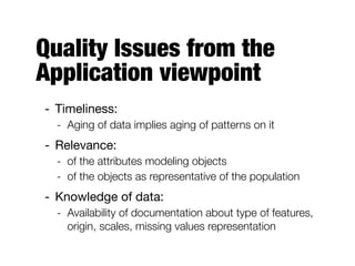
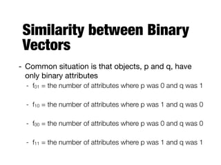
![Proximity
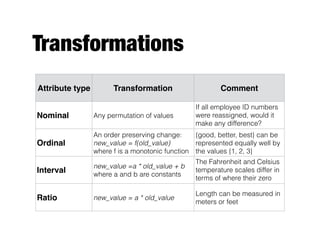
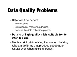
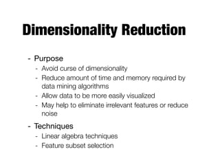
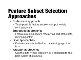
- Proximity refers to either similarity or
dissimilarity between two objects
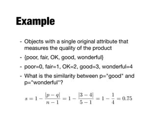
- Similarity
- Numerical measure of how alike two data objects are;
higher when objects are more alike
- Often falls in the range [0,1]
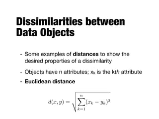
- Dissimilarity
- Numerical measure of how different are two data
objects; lower when objects are more alike
- Falls in the interval [0,1] or [0,infinity)](https://image.slidesharecdn.com/20170911-dat630-1-200214165218/85/Data-Mining-Introduction-and-Data-54-320.jpg)
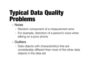
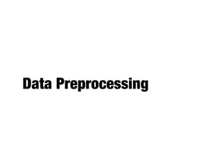
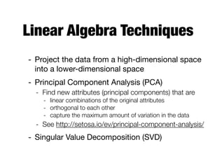
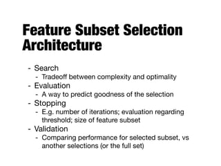
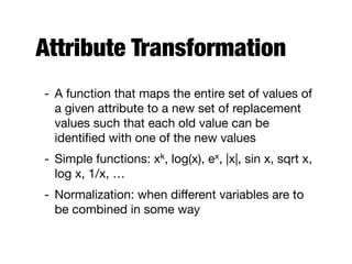
![Transformations
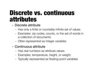
- To convert a similarity to a dissimilarity or vice
versa
- To transform a proximity measure to fall within
a certain range (e.g., [0,1])
- Min-max normalization
s0
=
s mins
maxs mins](https://image.slidesharecdn.com/20170911-dat630-1-200214165218/85/Data-Mining-Introduction-and-Data-55-320.jpg)


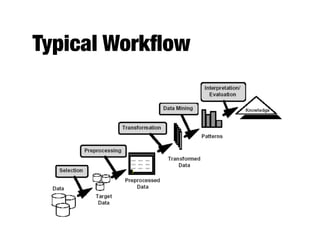
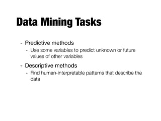
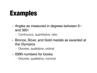
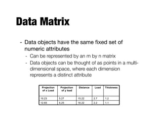
The document provides an introduction to data mining, outlining the process of extracting useful information from large datasets through exploration and analysis. It discusses various challenges, such as high dimensionality and data integration, as well as different data types and preprocessing techniques necessary to prepare data for effective mining. Key concepts include predictive and descriptive methods, data quality issues, and how to measure proximity between data objects.


![Wk. 3. Data [12-05-2021] (2).ppt](https://cdn.slidesharecdn.com/ss_thumbnails/wk-240205070901-8f81e253-thumbnail.jpg?width=640&height=640&fit=bounds)


![Polymer [ बहुलक ] Chemistry Notes PDF - Irfanullah Mehar - JJ Sir Chemistry.pdf](https://cdn.slidesharecdn.com/ss_thumbnails/polymerchemistrynotespdf-irfanullahmehar-jjsirchemistry-260210172118-3f9b37f7-thumbnail.jpg?width=640&height=640&fit=bounds)


