Data mining

1. Topic 2: Data Pre-processing
Julia Rahman
Data Mining
Course No: CSE 4221

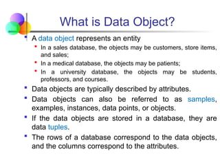
2. What is Data Object?
 A data object represents an entity
 In a sales database, the objects may be customers, store items,
and sales;
 In a medical database, the objects may be patients;
 In a university database, the objects may be students,
professors, and courses.
 Data objects are typically described by attributes.
 Data objects can also be referred to as samples,
examples, instances, data points, or objects.
 If the data objects are stored in a database, they are
data tuples.
 The rows of a database correspond to the data objects,
and the columns correspond to the attributes.

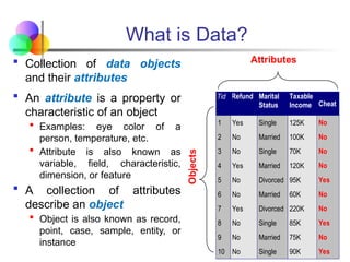
3. What is Data?
 Collection of data objects
and their attributes
 An attribute is a property or
characteristic of an object
 Examples: eye color of a
person, temperature, etc.
 Attribute is also known as
variable, field, characteristic,
dimension, or feature
 A collection of attributes
describe an object
 Object is also known as record,
point, case, sample, entity, or
instance
Tid Refund Marital
Status
Taxable
Income Cheat
1 Yes Single 125K No
2 No Married 100K No
3 No Single 70K No
4 Yes Married 120K No
5 No Divorced 95K Yes
6 No Married 60K No
7 Yes Divorced 220K No
8 No Single 85K Yes
9 No Married 75K No
10 No Single 90K Yes
10
Attributes
Objects

4. A More Complete View of Data
 Data may have parts
 The different parts of the data may have relationships
 More generally, data may have structure
 Data can be incomplete

5. Attribute Values
 Attribute values are numbers or symbols assigned to an
attribute for a particular object
 Distinction between attributes and attribute values
 Same attribute can be mapped to different attribute values
 Example: height can be measured in feet or meters
 Different attributes can be mapped to the same set of
values
 Example: Attribute values for ID and age are integers
 But properties of attribute values can be different

6. Types of Attributes
 There are different types of attributes
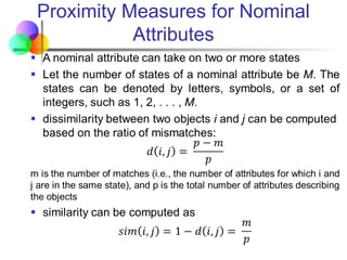
 Nominal
 Nominal means “relating to names.”
 The values of a nominal attribute are symbols or names of
things.
 Values are categorical.
 Examples: ID numbers, eye color, zip codes
 Ordinal
 An ordinal attribute is an attribute with possible values that
have a meaningful order or ranking among them.
 Examples: rankings (e.g., taste of potato chips on a scale from
1-10), grades, height {tall, medium, short}

7. Types of Attributes
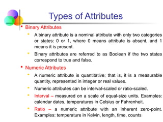
 Binary Attributes
 A binary attribute is a nominal attribute with only two categories
or states: 0 or 1, where 0 means attribute is absent, and 1
means it is present.
 Binary attributes are referred to as Boolean if the two states
correspond to true and false.
 Numeric Attributes
 A numeric attribute is quantitative; that is, it is a measurable
quantity, represented in integer or real values.
 Numeric attributes can be interval-scaled or ratio-scaled.
 Interval – measured on a scale of equal-size units. Examples:
calendar dates, temperatures in Celsius or Fahrenheit.
 Ratio – a numeric attribute with an inherent zero-point.
Examples: temperature in Kelvin, length, time, counts

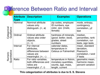
8. Difference Between Ratio and Interval
Attribute
Type
Description Examples Operations
Categorical
Qualitative
Nominal Nominal attribute
values only
distinguish. (=, 
)
zip codes, employee
ID numbers, eye
color, sex: {male,
female}
mode, entropy,
contingency
correlation, 2
test
Ordinal Ordinal attribute
values also order
objects.
(<, >)
hardness of minerals,
{good, better, best},
grades, street
numbers
median,
percentiles, rank
correlation, run
tests, sign tests
Numeric
Quantitative
Interval For interval
attributes,
differences between
values are
meaningful. (+, - )
calendar dates,
temperature in
Celsius or Fahrenheit
mean, standard
deviation,
Pearson's
correlation, t and
F tests
Ratio For ratio variables,
both differences and
ratios are
meaningful. (*, /)
temperature in Kelvin,
monetary quantities,
counts, age, mass,
length, current
geometric mean,
harmonic mean,
percent variation
This categorization of attributes is due to S. S. Stevens

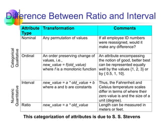
9. Difference Between Ratio and Interval
Attribute
Type
Transformation Comments
Categorical
Qualitative
Nominal Any permutation of values If all employee ID numbers
were reassigned, would it
make any difference?
Ordinal An order preserving change of
values, i.e.,
new_value = f(old_value)
where f is a monotonic function
An attribute encompassing
the notion of good, better best
can be represented equally
well by the values {1, 2, 3} or
by { 0.5, 1, 10}.
Numeric
Quantitative
Interval new_value = a * old_value + b
where a and b are constants
Thus, the Fahrenheit and
Celsius temperature scales
differ in terms of where their
zero value is and the size of a
unit (degree).
Ratio new_value = a * old_value Length can be measured in
meters or feet.
This categorization of attributes is due to S. S. Stevens

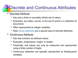
10. Discrete and Continuous Attributes
 Discrete Attribute
 Has only a finite or countably infinite set of values
 Examples: zip codes, counts, or the set of words in a collection of
documents
 Often represented as integer variables.
 Note: binary attributes are a special case of discrete attributes
 Continuous Attribute
 Has real numbers as attribute values
 Examples: temperature, height, or weight.
 Practically, real values can only be measured and represented
using a finite number of digits.
 Continuous attributes are typically represented as floating-point
variables.

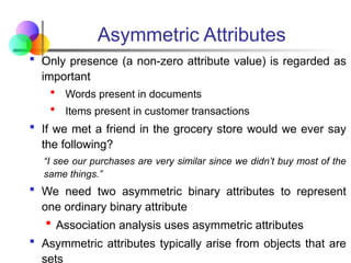
11. Asymmetric Attributes
 Only presence (a non-zero attribute value) is regarded as
important
 Words present in documents
 Items present in customer transactions
 If we met a friend in the grocery store would we ever say
the following?
“I see our purchases are very similar since we didn’t buy most of the
same things.”
 We need two asymmetric binary attributes to represent
one ordinary binary attribute
 Association analysis uses asymmetric attributes
 Asymmetric attributes typically arise from objects that are
sets

12. Types of data sets
 Record
 Data Matrix
 Document Data
 Transaction Data
 Graph
 World Wide Web
 Molecular Structures
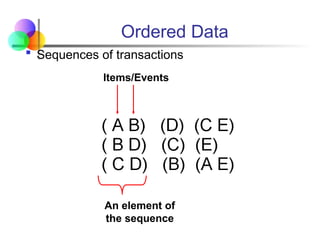
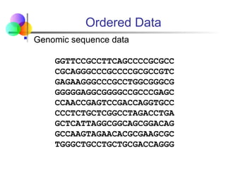
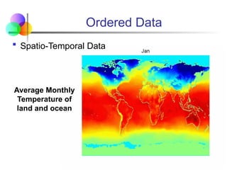
 Ordered
 Spatial Data
 Temporal Data
 Sequential Data
 Genetic Sequence Data

13. Important Characteristics of Data
 Dimensionality (number of attributes)
 High dimensional data brings a number of
challenges
 Sparsity
 Only presence counts
 Resolution
 Patterns depend on the scale
 Size
 Type of analysis may depend on size of data

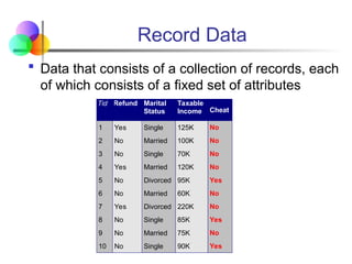
14. Record Data
 Data that consists of a collection of records, each
of which consists of a fixed set of attributes
Tid Refund Marital
Status
Taxable
Income Cheat
1 Yes Single 125K No
2 No Married 100K No
3 No Single 70K No
4 Yes Married 120K No
5 No Divorced 95K Yes
6 No Married 60K No
7 Yes Divorced 220K No
8 No Single 85K Yes
9 No Married 75K No
10 No Single 90K Yes
10

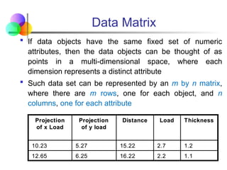
15. Data Matrix
 If data objects have the same fixed set of numeric
attributes, then the data objects can be thought of as
points in a multi-dimensional space, where each
dimension represents a distinct attribute
 Such data set can be represented by an m by n matrix,
where there are m rows, one for each object, and n
columns, one for each attribute
1.1
2.2
16.22
6.25
12.65
1.2
2.7
15.22
5.27
10.23
Thickness
Load
Distance
Projection
of y load
Projection
of x Load
1.1
2.2
16.22
6.25
12.65
1.2
2.7
15.22
5.27
10.23
Thickness
Load
Distance
Projection
of y load
Projection
of x Load

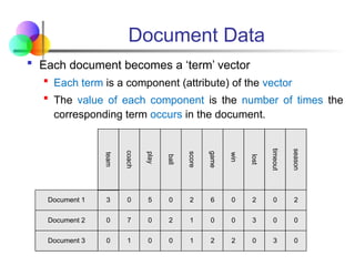
16. Document Data
 Each document becomes a ‘term’ vector
 Each term is a component (attribute) of the vector
 The value of each component is the number of times the
corresponding term occurs in the document.
Document 1
season
timeout
lost
win
game
score
ball
play
coach
team
Document 2
Document 3
3 0 5 0 2 6 0 2 0 2
0
0
7 0 2 1 0 0 3 0 0
1 0 0 1 2 2 0 3 0

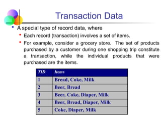
17. Transaction Data
 A special type of record data, where
 Each record (transaction) involves a set of items.
 For example, consider a grocery store. The set of products
purchased by a customer during one shopping trip constitute
a transaction, while the individual products that were
purchased are the items.
TID Items
1 Bread, Coke, Milk
2 Beer, Bread
3 Beer, Coke, Diaper, Milk
4 Beer, Bread, Diaper, Milk
5 Coke, Diaper, Milk

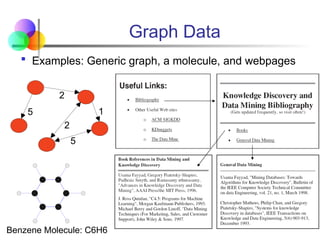
18. Graph Data
 Examples: Generic graph, a molecule, and webpages
5
2
1
2
5
Benzene Molecule: C6H6

19. Ordered Data
 Sequences of transactions
An element of
the sequence
Items/Events

20. Ordered Data
 Genomic sequence data
GGTTCCGCCTTCAGCCCCGCGCC
CGCAGGGCCCGCCCCGCGCCGTC
GAGAAGGGCCCGCCTGGCGGGCG
GGGGGAGGCGGGGCCGCCCGAGC
CCAACCGAGTCCGACCAGGTGCC
CCCTCTGCTCGGCCTAGACCTGA
GCTCATTAGGCGGCAGCGGACAG
GCCAAGTAGAACACGCGAAGCGC
TGGGCTGCCTGCTGCGACCAGGG

21. Ordered Data
 Spatio-Temporal Data
Average Monthly
Temperature of
land and ocean

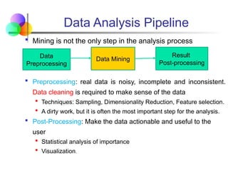
22. Data Analysis Pipeline
 Mining is not the only step in the analysis process
 Preprocessing: real data is noisy, incomplete and inconsistent.
Data cleaning is required to make sense of the data
 Techniques: Sampling, Dimensionality Reduction, Feature selection.
 A dirty work, but it is often the most important step for the analysis.
 Post-Processing: Make the data actionable and useful to the
user
 Statistical analysis of importance
 Visualization.
Data
Preprocessing
Data Mining
Result
Post-processing

23. Why Data Preprocessing?
 Measures for data quality: A multidimensional view
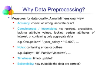
 Accuracy: correct or wrong, accurate or not
 Completeness / Incomplete: not recorded, unavailable,
lacking attribute values, lacking certain attributes of
interest, or containing only aggregate data
e.g. Occupation=“ ”, year_salary = “13.000”, …
 Noisy: containing errors or outliers
e.g. Salary=“-10”, Family=“Unknown”, …
 Timeliness: timely update?
 Believability: how trustable the data are correct?

24. Why Data Preprocessing?
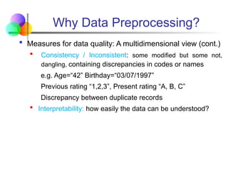
 Measures for data quality: A multidimensional view (cont.)
 Consistency / Inconsistent: some modified but some not,
dangling, containing discrepancies in codes or names
e.g. Age=“42” Birthday=“03/07/1997”
Previous rating “1,2,3”, Present rating “A, B, C”
Discrepancy between duplicate records
 Interpretability: how easily the data can be understood?

25. Why data is dirty?
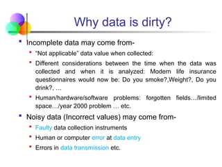
 Incomplete data may come from-
 “Not applicable” data value when collected:
 Different considerations between the time when the data was
collected and when it is analyzed: Modern life insurance
questionnaires would now be: Do you smoke?,Weight?, Do you
drink?, …
 Human/hardware/software problems: forgotten fields…/limited
space…/year 2000 problem … etc.
 Noisy data (Incorrect values) may come from-
 Faulty data collection instruments
 Human or computer error at data entry
 Errors in data transmission etc.

26. Why data is dirty?
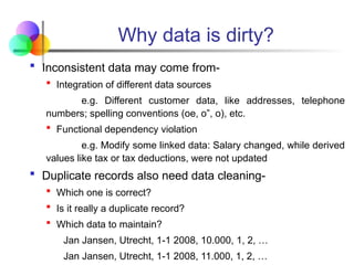
 Inconsistent data may come from-
 Integration of different data sources
e.g. Different customer data, like addresses, telephone
numbers; spelling conventions (oe, o”, o), etc.
 Functional dependency violation
e.g. Modify some linked data: Salary changed, while derived
values like tax or tax deductions, were not updated
 Duplicate records also need data cleaning-
 Which one is correct?
 Is it really a duplicate record?
 Which data to maintain?
Jan Jansen, Utrecht, 1-1 2008, 10.000, 1, 2, …
Jan Jansen, Utrecht, 1-1 2008, 11.000, 1, 2, …

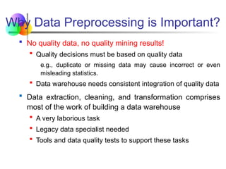
27. Why Data Preprocessing is Important?
 No quality data, no quality mining results!
 Quality decisions must be based on quality data
e.g., duplicate or missing data may cause incorrect or even
misleading statistics.
 Data warehouse needs consistent integration of quality data
 Data extraction, cleaning, and transformation comprises
most of the work of building a data warehouse
 A very laborious task
 Legacy data specialist needed
 Tools and data quality tests to support these tasks

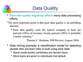
28. Data Quality
 Poor data quality negatively affects many data processing
efforts
“The most important point is that poor data quality is an unfolding
disaster.
 Poor data quality costs the typical company at least ten
percent (10%) of revenue; twenty percent (20%) is probably
a better estimate.”
Thomas C. Redman, DM Review, August 2004
 Data mining example: a classification model for detecting
people who are loan risks is built using poor data
 Some credit-worthy candidates are denied loans
 More loans are given to individuals that default

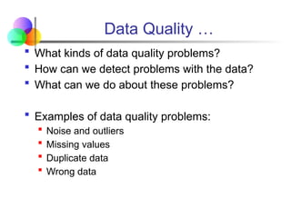
29. Data Quality …
 What kinds of data quality problems?
 How can we detect problems with the data?
 What can we do about these problems?
 Examples of data quality problems:
 Noise and outliers
 Missing values
 Duplicate data
 Wrong data

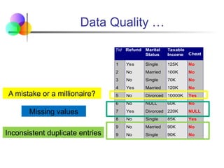
30. Data Quality …
Tid Refund Marital
Status
Taxable
Income Cheat
1 Yes Single 125K No
2 No Married 100K No
3 No Single 70K No
4 Yes Married 120K No
5 No Divorced 10000K Yes
6 No NULL 60K No
7 Yes Divorced 220K NULL
8 No Single 85K Yes
9 No Married 90K No
9 No Single 90K No
10
A mistake or a millionaire?
Missing values
Inconsistent duplicate entries

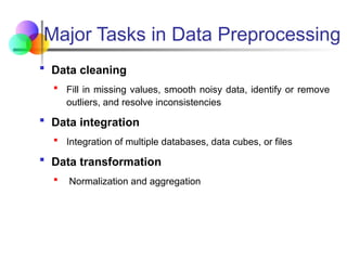
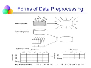
31. Major Tasks in Data Preprocessing
 Data cleaning
 Fill in missing values, smooth noisy data, identify or remove
outliers, and resolve inconsistencies
 Data integration
 Integration of multiple databases, data cubes, or files
 Data transformation
 Normalization and aggregation

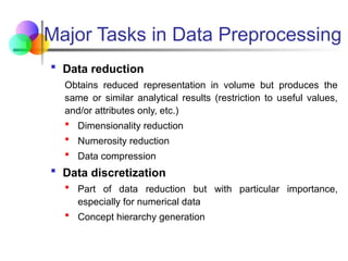
32. Major Tasks in Data Preprocessing
 Data reduction
Obtains reduced representation in volume but produces the
same or similar analytical results (restriction to useful values,
and/or attributes only, etc.)
 Dimensionality reduction
 Numerosity reduction
 Data compression
 Data discretization
 Part of data reduction but with particular importance,
especially for numerical data
 Concept hierarchy generation

33. Forms of Data Preprocessing

34. Mining Data Descriptive Characteristics
 Motivation
 To better understand the data
 To highlight which data values should be treated as noise or
outliers.
 Data dispersion characteristics
 median, max, min, quantiles, outliers, variance, etc.
 Numerical dimensions correspond to sorted intervals
 Data dispersion: analyzed with multiple granularities of
precision
 Boxplot or quantile analysis on sorted intervals
 Dispersion analysis on computed measures
 Folding measures into numerical dimensions
 Boxplot or quantile analysis on the transformed cube

35. Measuring the Central Tendency
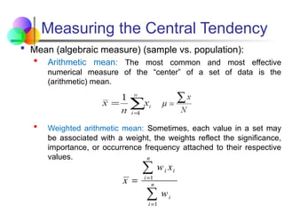
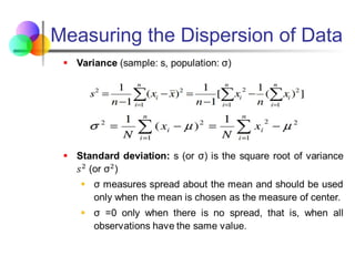
 Mean (algebraic measure) (sample vs. population):
 Arithmetic mean: The most common and most effective
numerical measure of the “center” of a set of data is the
(arithmetic) mean.
 Weighted arithmetic mean: Sometimes, each value in a set may
be associated with a weight, the weights reflect the significance,
importance, or occurrence frequency attached to their respective
values.

36. Measuring the Central Tendency
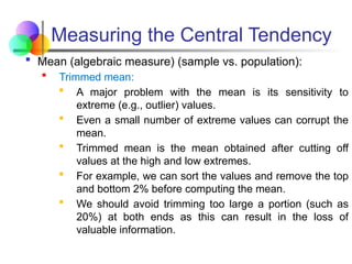
 Mean (algebraic measure) (sample vs. population):
 Trimmed mean:
 A major problem with the mean is its sensitivity to
extreme (e.g., outlier) values.
 Even a small number of extreme values can corrupt the
mean.
 Trimmed mean is the mean obtained after cutting off
values at the high and low extremes.
 For example, we can sort the values and remove the top
and bottom 2% before computing the mean.
 We should avoid trimming too large a portion (such as
20%) at both ends as this can result in the loss of
valuable information.

37. Measuring the Central Tendency
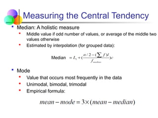
 Median: A holistic measure
 Middle value if odd number of values, or average of the middle two
values otherwise
 Estimated by interpolation (for grouped data):
Median
 Mode
 Value that occurs most frequently in the data
 Unimodal, bimodal, trimodal
 Empirical formula:

38. Symmetric vs. Skewed Data
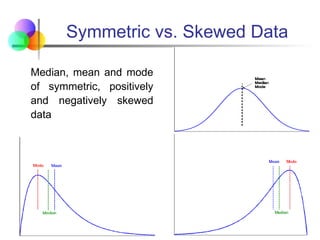
Median, mean and mode
of symmetric, positively
and negatively skewed
data

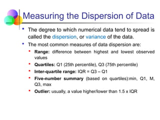
39. Measuring the Dispersion of Data
 The degree to which numerical data tend to spread is
called the dispersion, or variance of the data.
 The most common measures of data dispersion are:
 Range: difference between highest and lowest observed
values
 Quartiles: Q1 (25th percentile), Q3 (75th percentile)
 Inter-quartile range: IQR = Q3 – Q1
 Five-number summary (based on quartiles):min, Q1, M,
Q3, max
 Outlier: usually, a value higher/lower than 1.5 x IQR

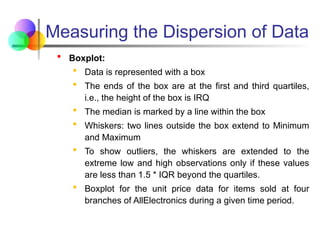
40. Measuring the Dispersion of Data
 Boxplot:
 Data is represented with a box
 The ends of the box are at the first and third quartiles,
i.e., the height of the box is IRQ
 The median is marked by a line within the box
 Whiskers: two lines outside the box extend to Minimum
and Maximum
 To show outliers, the whiskers are extended to the
extreme low and high observations only if these values
are less than 1.5 * IQR beyond the quartiles.
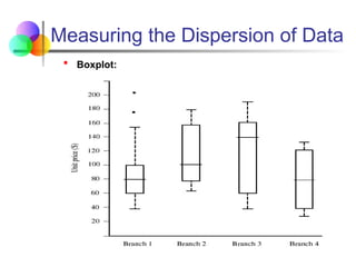
 Boxplot for the unit price data for items sold at four
branches of AllElectronics during a given time period.

41. Measuring the Dispersion of Data
 Boxplot:

42. Measuring the Dispersion of Data

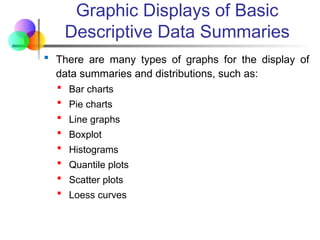
43. Graphic Displays of Basic
Descriptive Data Summaries
 There are many types of graphs for the display of
data summaries and distributions, such as:
 Bar charts
 Pie charts
 Line graphs
 Boxplot
 Histograms
 Quantile plots
 Scatter plots
 Loess curves

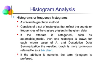
44. Histogram Analysis
 Histograms or frequency histograms
 A univariate graphical method
 Consists of a set of rectangles that reflect the counts or
frequencies of the classes present in the given data
 If the attribute is categorical, such as
automobile_model, then one rectangle is drawn for
each known value of A, and Descriptive Data
Summarization the resulting graph is more commonly
referred to as a bar chart.
 If the attribute is numeric, the term histogram is
preferred.

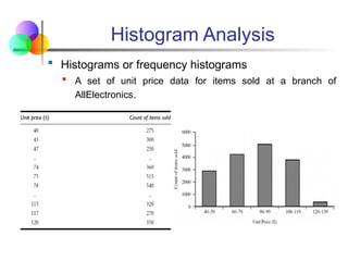
45. Histogram Analysis
 Histograms or frequency histograms
 A set of unit price data for items sold at a branch of
AllElectronics.

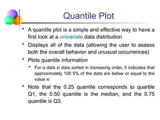
46. Quantile Plot
 A quantile plot is a simple and effective way to have a
first look at a univariate data distribution
 Displays all of the data (allowing the user to assess
both the overall behavior and unusual occurrences)
 Plots quantile information
 For a data xi data sorted in increasing order, fi indicates that
approximately 100 fi% of the data are below or equal to the
value xi
 Note that the 0.25 quantile corresponds to quartile
Q1, the 0.50 quantile is the median, and the 0.75
quantile is Q3.

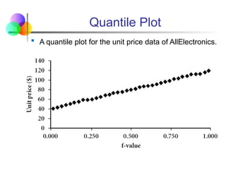
47. Quantile Plot
 A quantile plot for the unit price data of AllElectronics.

48. Scatter plot
 A scatter plot is one of the most effective graphical
methods for determining if there appears to be a
relationship, clusters of points, or outliers between
two numerical attributes.
 Each pair of values is treated as a pair of coordinates
and plotted as points in the plane

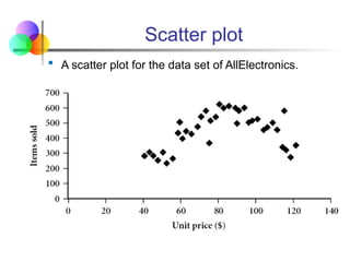
49. Scatter plot
 A scatter plot for the data set of AllElectronics.

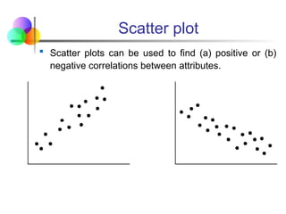
50. Scatter plot
 Scatter plots can be used to find (a) positive or (b)
negative correlations between attributes.

51. Scatter plot
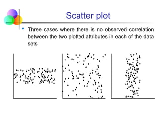
 Three cases where there is no observed correlation
between the two plotted attributes in each of the data
sets

52. Loess Curve
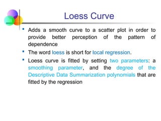
 Adds a smooth curve to a scatter plot in order to
provide better perception of the pattern of
dependence
 The word loess is short for local regression.
 Loess curve is fitted by setting two parameters: a
smoothing parameter, and the degree of the
Descriptive Data Summarization polynomials that are
fitted by the regression

53. Loess Curve
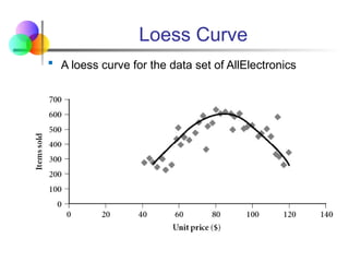
 A loess curve for the data set of AllElectronics

54. Data Cleaning
 Why Data Cleaning?
 “Data cleaning is one of the three biggest problems in data
warehousing”—Ralph Kimball
 “Data cleaning is the number one problem in data
warehousing”—DCI survey
 Data cleaning tasks
 Fill in missing values
 Identify outliers and smooth out noisy data
 Correct inconsistent data
 Resolve redundancy caused by data integration

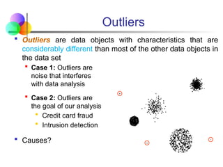
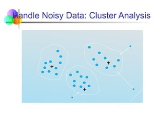
55. Outliers
 Outliers are data objects with characteristics that are
considerably different than most of the other data objects in
the data set
 Case 1: Outliers are
noise that interferes
with data analysis
 Case 2: Outliers are
the goal of our analysis
 Credit card fraud
 Intrusion detection
 Causes?

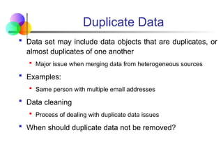
56. Duplicate Data
 Data set may include data objects that are duplicates, or
almost duplicates of one another
 Major issue when merging data from heterogeneous sources
 Examples:
 Same person with multiple email addresses
 Data cleaning
 Process of dealing with duplicate data issues
 When should duplicate data not be removed?

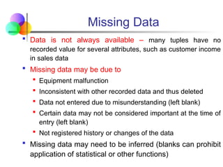
57. Missing Data
 Data is not always available – many tuples have no
recorded value for several attributes, such as customer income
in sales data
 Missing data may be due to
 Equipment malfunction
 Inconsistent with other recorded data and thus deleted
 Data not entered due to misunderstanding (left blank)
 Certain data may not be considered important at the time of
entry (left blank)
 Not registered history or changes of the data
 Missing data may need to be inferred (blanks can prohibit
application of statistical or other functions)

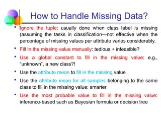
58. How to Handle Missing Data?
 Ignore the tuple: usually done when class label is missing
(assuming the tasks in classification—not effective when the
percentage of missing values per attribute varies considerably.
 Fill in the missing value manually: tedious + infeasible?
 Use a global constant to fill in the missing value: e.g.,
“unknown”, a new class?!
 Use the attribute mean to fill in the missing value
 Use the attribute mean for all samples belonging to the same
class to fill in the missing value: smarter
 Use the most probable value to fill in the missing value:
inference-based such as Bayesian formula or decision tree

59. Noisy Data
 Noise: Random error or variance in a measured variable
 Incorrect attribute values may be due to
 Faulty data collection instruments
 Data entry problems
 Data transmission problems
 Technology limitation
 Inconsistency in naming convention (H. Shree, HShree,
H.Shree, H Shree etc.)
 Other data problems which requires data cleaning
 Duplicate records (omit duplicates)
 Incomplete data (interpolate, estimate, etc.)
 Inconsistent data (decide which one is correct …)

60. How to Handle Noisy Data?
 Binning
 Groups or divides continuous data into a series of small
intervals, called "bins," and replaces the values within each
bin by a representative value.
 Regression
 Smooth by fitting the data into regression functions
 Clustering
 Detect and remove outliers
 Combined computer and human inspection
 Detect suspicious values and check by human (e.g., deal
with possible outliers)

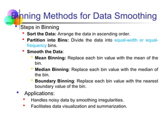
61.  Steps in Binning
 Sort the Data: Arrange the data in ascending order.
 Partition into Bins: Divide the data into equal-width or equal-
frequency bins.
 Smooth the Data:
 Mean Binning: Replace each bin value with the mean of the
bin.
 Median Binning: Replace each bin value with the median of
the bin.
 Boundary Binning: Replace each bin value with the nearest
boundary value of the bin.
 Applications:
 Handles noisy data by smoothing irregularities.
 Facilitates data visualization and summarization.
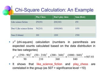
Binning Methods for Data Smoothing

62. Binning Methods for Data Smoothing
 Sorted data for price (in dollars): 4, 8, 9, 15, 21, 21, 24,
25, 26, 28, 29, 34
 Partition into equal-frequency (equal width) bins:
- Bin 1: [4, 8, 9, 15]
- Bin 2: [21, 21, 24, 25]
- Bin 3: [26, 28, 29, 34]
 Smoothing by bin means: [9, 9, 9, 9], [23, 23, 23, 23], [29,
29, 29, 29]
 Smoothing by bin median : [8.5, 8.5, 8.5, 8.5], [22.5, 22.5,
22.5, 22.5], [28.5, 28.5, 28.5, 28.5]
 Smoothing by bin boundaries: [4, 4, 4, 15] (*boundaries 4 and
15, report closest boundary), [21, 21, 25, 25], [26, 26, 26, 34]

63. Handle Noisy Data: Cluster Analysis

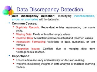
64. Data Discrepancy Detection
 Data Discrepancy Detection: Identifying inconsistencies,
errors, or anomalies within datasets.
 Common Causes:
 Duplicate Records: Redundant entries representing the same
entity.
 Missing Data: Fields with null or empty values.
 Incorrect Data: Mismatches between actual and recorded values.
 Inconsistent Formatting: Variations in date, numerical, or text
formats.
 Integration Issues: Conflicts due to merging data from
heterogeneous sources.
 Importance:
 Ensures data accuracy and reliability for decision-making.
 Prevents misleading insights in data analysis or machine learning
models.

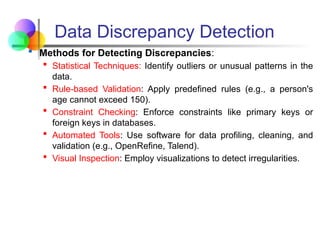
65. Data Discrepancy Detection
 Methods for Detecting Discrepancies:
 Statistical Techniques: Identify outliers or unusual patterns in the
data.
 Rule-based Validation: Apply predefined rules (e.g., a person's
age cannot exceed 150).
 Constraint Checking: Enforce constraints like primary keys or
foreign keys in databases.
 Automated Tools: Use software for data profiling, cleaning, and
validation (e.g., OpenRefine, Talend).
 Visual Inspection: Employ visualizations to detect irregularities.

66. Data Cleaning Process
 Data migration and integration
 Data migration tools: allow transformations to be specified
 ETL (Extraction/Transformation/Loading) tools: allow
users to specify transformations through a graphical user
interface
 Integration of the two processes
 Iterative and interactive (e.g., Potter’s Wheels)

67. Data Integration and Transformation
 Data integration
 Combines data from multiple sources into a coherent store
 Schema integration:
 Integrate metadata from different sources
 e.g., A.cust-id B.cust-#

 Entity identification problem
 Identify and use real world entities from multiple data
sources, e.g., Bill Clinton = William Clinton
 Detecting and resolving data value conflicts
 For the same real-world entity, attribute values from different
sources are different
 Possible reasons: different representations, different scales,
e.g., metric vs. British units

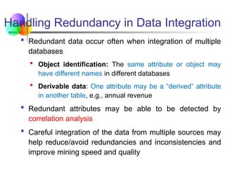
68. Handling Redundancy in Data Integration
 Redundant data occur often when integration of multiple
databases
 Object identification: The same attribute or object may
have different names in different databases
 Derivable data: One attribute may be a “derived” attribute
in another table, e.g., annual revenue
 Redundant attributes may be able to be detected by
correlation analysis
 Careful integration of the data from multiple sources may
help reduce/avoid redundancies and inconsistencies and
improve mining speed and quality

69. Correlation Analysis (Numerical Data)

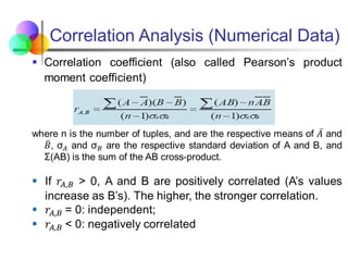
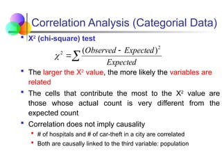
70. Correlation Analysis (Categorial Data)
 Χ2
(chi-square) test
 The larger the Χ2
value, the more likely the variables are
related
 The cells that contribute the most to the Χ2
value are
those whose actual count is very different from the
expected count
 Correlation does not imply causality
 # of hospitals and # of car-theft in a city are correlated
 Both are causally linked to the third variable: population



Expected
Expected
Observed 2
2 )
(


71. Chi-Square Calculation: An Example
93
.
507
840
)
840
1000
(
360
)
360
200
(
210
)
210
50
(
90
)
90
250
( 2
2
2
2
2











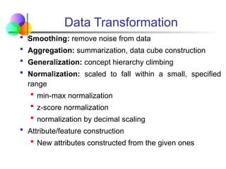
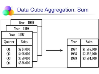
72. Data Transformation
 Smoothing: remove noise from data
 Aggregation: summarization, data cube construction
 Generalization: concept hierarchy climbing
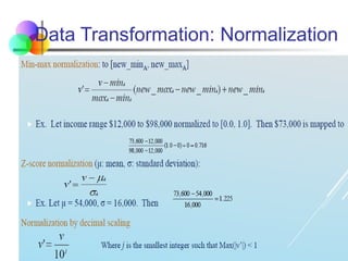
 Normalization: scaled to fall within a small, specified
range
 min-max normalization
 z-score normalization
 normalization by decimal scaling
 Attribute/feature construction
 New attributes constructed from the given ones

73. Data Transformation: Normalization

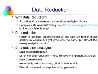
74.  Why Data Reduction?
 A database/data warehouse may store terabytes of data
 Complex data analysis/mining may take a very long time to run
on the complete data set
 Data reduction
 Obtain a reduced representation of the data set that is much
smaller in volume but yet produces the same (or almost the
same) analytical results
 Data reduction strategies
 Data cube aggregation:
 Dimensionality reduction — e.g., remove unimportant attributes
 Data Compression
 Numerosity reduction — e.g., fit data into models
 Discretization and concept hierarchy generation
Data Reduction

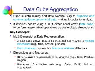
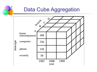
75.  Used in data mining and data warehousing to organize and
summarize large amounts of data, making it easier to analyze.
 It involves constructing a multi-dimensional array (data cube)
to perform aggregation operations across multiple dimensions.
Key Concepts:
 Multi-Dimensional Data Representation:
 A data cube allows data to be modelled and viewed in multiple
dimensions (e.g., time, location, product).
 Each dimension represents a feature or attribute of the data.
 Dimensions and Measures:
 Dimensions: The perspectives for analysis (e.g., Time, Product,
Region).
 Measures: Quantitative data (e.g., Sales, Profit) that are
aggregated.
Data Cube Aggregation

76. Data Cube Aggregation

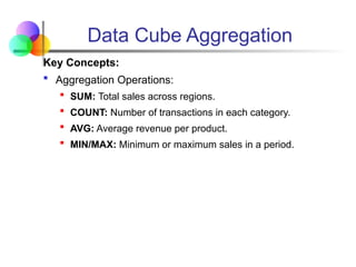
77. Key Concepts:
 Aggregation Operations:
 SUM: Total sales across regions.
 COUNT: Number of transactions in each category.
 AVG: Average revenue per product.
 MIN/MAX: Minimum or maximum sales in a period.
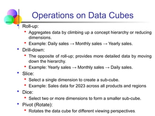
Data Cube Aggregation

78. Data Cube Aggregation: Sum

79.  Roll-up:
 Aggregates data by climbing up a concept hierarchy or reducing
dimensions.
 Example: Daily sales → Monthly sales → Yearly sales.
 Drill-down:
 The opposite of roll-up; provides more detailed data by moving
down the hierarchy.
 Example: Yearly sales → Monthly sales → Daily sales.
 Slice:
 Select a single dimension to create a sub-cube.
 Example: Sales data for 2023 across all products and regions
 Dice:
 Select two or more dimensions to form a smaller sub-cube.
 Pivot (Rotate):
 Rotates the data cube for different viewing perspectives.
Operations on Data Cubes

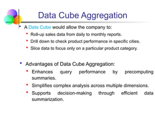
80.  A Data Cube would allow the company to:
 Roll-up sales data from daily to monthly reports.
 Drill down to check product performance in specific cities.
 Slice data to focus only on a particular product category.
 Advantages of Data Cube Aggregation:
 Enhances query performance by precomputing
summaries.
 Simplifies complex analysis across multiple dimensions.
 Supports decision-making through efficient data
summarization.
Data Cube Aggregation

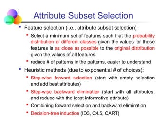
81.  Feature selection (i.e., attribute subset selection):
 Select a minimum set of features such that the probability
distribution of different classes given the values for those
features is as close as possible to the original distribution
given the values of all features
 reduce # of patterns in the patterns, easier to understand
 Heuristic methods (due to exponential # of choices):
 Step-wise forward selection (start with empty selection
and add best attributes)
 Step-wise backward elimination (start with all attributes,
and reduce with the least informative attribute)
 Combining forward selection and backward elimination
 Decision-tree induction (ID3, C4.5, CART)
Attribute Subset Selection

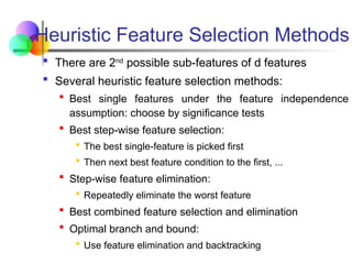
82.  There are 2nd
possible sub-features of d features
 Several heuristic feature selection methods:
 Best single features under the feature independence
assumption: choose by significance tests
 Best step-wise feature selection:
 The best single-feature is picked first
 Then next best feature condition to the first, ...
 Step-wise feature elimination:
 Repeatedly eliminate the worst feature
 Best combined feature selection and elimination
 Optimal branch and bound:
 Use feature elimination and backtracking
Heuristic Feature Selection Methods

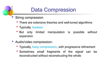
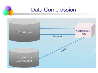
83.  String compression
 There are extensive theories and well-tuned algorithms
 Typically, lossless
 But only limited manipulation is possible without
expansion
 Audio/video compression:
 Typically, lossy compression, with progressive refinement
 Sometimes small fragments of the signal can be
reconstructed without reconstructing the whole
Data Compression

84. Data Compression

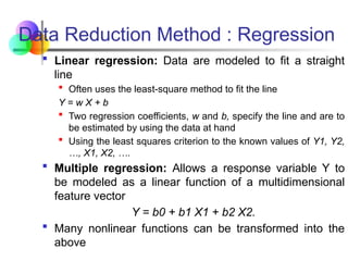
85.  Linear regression: Data are modeled to fit a straight
line
 Often uses the least-square method to fit the line
Y = w X + b
 Two regression coefficients, w and b, specify the line and are to
be estimated by using the data at hand
 Using the least squares criterion to the known values of Y1, Y2,
…, X1, X2, ….
 Multiple regression: Allows a response variable Y to
be modeled as a linear function of a multidimensional
feature vector
Y = b0 + b1 X1 + b2 X2.
 Many nonlinear functions can be transformed into the
above
Data Reduction Method : Regression

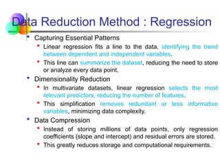
86.  Capturing Essential Patterns
 Linear regression fits a line to the data, identifying the trend
between dependent and independent variables.
 This line can summarize the dataset, reducing the need to store
or analyze every data point.
 Dimensionality Reduction
 In multivariate datasets, linear regression selects the most
relevant predictors, reducing the number of features.
 This simplification removes redundant or less informative
variables, minimizing data complexity.
 Data Compression
 Instead of storing millions of data points, only regression
coefficients (slope and intercept) and residual errors are stored.
 This greatly reduces storage and computational requirements.
Data Reduction Method : Regression

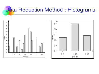
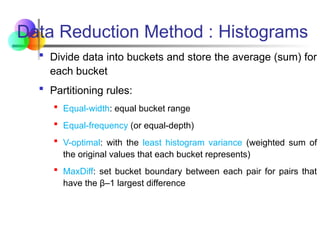
87.  Divide data into buckets and store the average (sum) for
each bucket
 Partitioning rules:
 Equal-width: equal bucket range
 Equal-frequency (or equal-depth)
 V-optimal: with the least histogram variance (weighted sum of
the original values that each bucket represents)
 MaxDiff: set bucket boundary between each pair for pairs that
have the β–1 largest difference
Data Reduction Method : Histograms

88. Data Reduction Method : Histograms

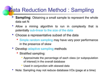
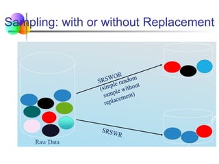
89.  Sampling: Obtaining a small sample to represent the whole
data set N
 Allow a mining algorithm to run in complexity that is
potentially sub-linear to the size of the data
 Choose a representative subset of the data
 Simple random sampling may have very poor performance
in the presence of skew
 Develop adaptive sampling methods
 Stratified sampling:
 Approximate the percentage of each class (or subpopulation
of interest) in the overall database
 Used in conjunction with skewed data
 Note: Sampling may not reduce database I/Os (page at a time)
Data Reduction Method : Sampling

90. Sampling: with or without Replacement

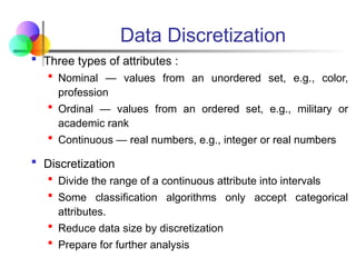
91. Data Discretization
 Three types of attributes :
 Nominal — values from an unordered set, e.g., color,
profession
 Ordinal — values from an ordered set, e.g., military or
academic rank
 Continuous — real numbers, e.g., integer or real numbers
 Discretization
 Divide the range of a continuous attribute into intervals
 Some classification algorithms only accept categorical
attributes.
 Reduce data size by discretization
 Prepare for further analysis

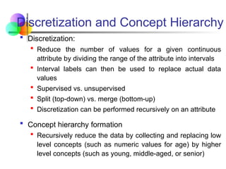
92. Discretization and Concept Hierarchy
 Discretization:
 Reduce the number of values for a given continuous
attribute by dividing the range of the attribute into intervals
 Interval labels can then be used to replace actual data
values
 Supervised vs. unsupervised
 Split (top-down) vs. merge (bottom-up)
 Discretization can be performed recursively on an attribute
 Concept hierarchy formation
 Recursively reduce the data by collecting and replacing low
level concepts (such as numeric values for age) by higher
level concepts (such as young, middle-aged, or senior)

93. Hierarchical Reduction

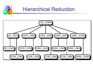
94. Discretization and Concept Hierarchy
Generation for Numeric Data
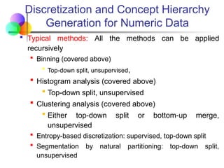
 Typical methods: All the methods can be applied
recursively
 Binning (covered above)
 Top-down split, unsupervised,
 Histogram analysis (covered above)
 Top-down split, unsupervised
 Clustering analysis (covered above)
 Either top-down split or bottom-up merge,
unsupervised
 Entropy-based discretization: supervised, top-down split
 Segmentation by natural partitioning: top-down split,
unsupervised

95. Similarity and Dissimilarity Measures
 Similarity measure
 Numerical measure of how alike two data objects are.
 Is higher when objects are more alike.
 Often falls in the range [0,1]
 Dissimilarity measure
 Numerical measure of how different two data objects are
 Lower when objects are more alike
 Minimum dissimilarity is often 0
 Upper limit varies
 Proximity refers to a similarity or dissimilarity
 Two data structures that are commonly used
 Data matrix (used to store the data objects) and
 Dissimilarity matrix (used to store dissimilarity values for pairs of
objects).

96. Data Matrix Vs Dissimilarity Matrix

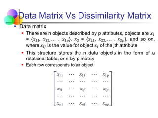
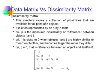
97. Data Matrix Vs Dissimilarity Matrix
 Dissimilarity matrix
 This structure stores a collection of proximities that are
available for all pairs of n objects.
 It is often represented by an n-by-n table
 d(i, j) is the measured dissimilarity or “difference” between
objects i and j.
 d(i, j) is close to 0 when objects i and j are highly similar or
“near” each other, and becomes larger the more they differ.
 d(i, i) = 0; that is difference between an object and itself is 0.

98. Proximity Measures for Nominal
Attributes

99. Proximity Measures for Binary
Attributes

100. Dissimilarity of Numeric Data
 Commonly used technique:
 Euclidean distance
 Manhattan distance, and
 Minkowski distances
 In some cases, the data are normalized before applying
distance calculations – transforming the data to fall within
a smaller or common range, such as [-1, 1] or [0.0, 1.0].

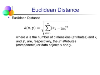
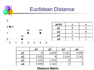
101. Euclidean Distance
 Euclidean Distance
where n is the number of dimensions (attributes) and xk
and yk are, respectively, the kth
attributes
(components) or data objects x and y.

102. Euclidean Distance
0
1
2
3
0 1 2 3 4 5 6
p1
p2
p3 p4
point x y
p1 0 2
p2 2 0
p3 3 1
p4 5 1
Distance Matrix
p1 p2 p3 p4
p1 0 2.828 3.162 5.099
p2 2.828 0 1.414 3.162
p3 3.162 1.414 0 2
p4 5.099 3.162 2 0

103. Manhattan Distance

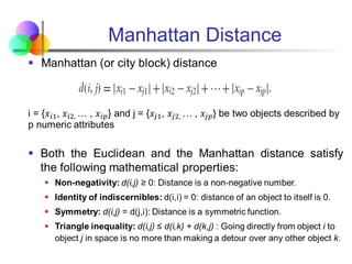
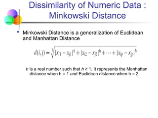
104. Dissimilarity of Numeric Data :
Minkowski Distance
 Minkowski Distance is a generalization of Euclidean
and Manhattan Distance
h is a real number such that h ≥ 1. It represents the Manhattan
distance when h = 1 and Euclidean distance when h = 2.

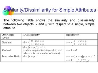
105. Similarity/Dissimilarity for Simple Attributes
The following table shows the similarity and dissimilarity
between two objects, x and y, with respect to a single, simple
attribute.

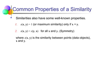
106. Common Properties of a Similarity
 Similarities also have some well-known properties.
1. s(x, y) = 1 (or maximum similarity) only if x = y.
2. s(x, y) = s(y, x) for all x and y. (Symmetry)
where s(x, y) is the similarity between points (data objects),
x and y.

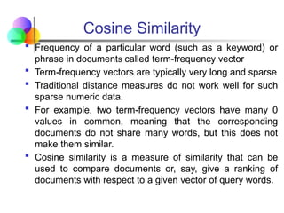
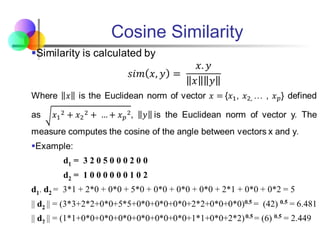
107. Cosine Similarity
 Frequency of a particular word (such as a keyword) or
phrase in documents called term-frequency vector
 Term-frequency vectors are typically very long and sparse
 Traditional distance measures do not work well for such
sparse numeric data.
 For example, two term-frequency vectors have many 0
values in common, meaning that the corresponding
documents do not share many words, but this does not
make them similar.
 Cosine similarity is a measure of similarity that can be
used to compare documents or, say, give a ranking of
documents with respect to a given vector of query words.

108. Cosine Similarity