بررسی دو روش شناسایی سیستم متغیر بازمان با جزییات و توضیحات ساده و گویا و توضیح روابط و علایم به طور کامل به همراه مثال و شبیه سازی در متلب و فایل های مرجع و مقالات مرجع
روش اول: شناسایی سیستم با پارامترهای متغیر با زمان با استفاده از Least Square
روش دوم: شناسایی سیستم دینامیکی با استفاده از شبکه های عصبی مصنوعی
مناسب برای ارائه به عنوان تحقیق یا پروژه درس شناسایی سیستم ها
به همراه شبیه سازی در متلب و گزارش 20 صفحه ای
https://www.prjmarket.com/product/%d8%a8%d8%b1%d8%b1%d8%b3%db%8c-%d8%af%d9%88-%d8%b1%d9%88%d8%b4-%d8%b4%d9%86%d8%a7%d8%b3%d8%a7%db%8c%db%8c-%d8%b3%db%8c%d8%b3%d8%aa%d9%85-%d9%87%d8%a7%db%8c-%d9%85%d8%aa%d8%ba%db%8c%d8%b1-%d8%a8%d8%a7/
This paper proposes modeling and identification of dynamical systems in delta
domain using neural network. The properties of delta operator are used such as greater
numerical robustness in computation and superior coefficients representation in finite word
length in implementation and well ensured numerical conditioning at high sampling
frequency. To formulate the identification scheme delta operator model is recasted into a
realizable neural network structure using the properties of inverse delta operator.
Presentation of my NSERC-USRA funded summer research project given at the Canadian Undergraduate Mathematics Conference (CUMC) 2014.
Please refer to the project site: http://jessebett.com/Radial-Basis-Function-USRA/
Tensor representations in signal processing and machine learning (tutorial ta...Tatsuya Yokota
Tutorial talk in APSIPA-ASC 2020.
Title: Tensor representations in signal processing and machine learning.
Introduction to tensor decomposition (テンソル分解入門)
Basics of tensor decomposition (テンソル分解の基礎)
https://telecombcn-dl.github.io/2018-dlai/
Deep learning technologies are at the core of the current revolution in artificial intelligence for multimedia data analysis. The convergence of large-scale annotated datasets and affordable GPU hardware has allowed the training of neural networks for data analysis tasks which were previously addressed with hand-crafted features. Architectures such as convolutional neural networks, recurrent neural networks or Q-nets for reinforcement learning have shaped a brand new scenario in signal processing. This course will cover the basic principles of deep learning from both an algorithmic and computational perspectives.
A Novel Methodology for Designing Linear Phase IIR FiltersIDES Editor
This paper presents a novel technique for
designing an Infinite Impulse Response (IIR) Filter with
Linear Phase Response. The design of IIR filter is always a
challenging task due to the reason that a Linear Phase
Response is not realizable in this kind. The conventional
techniques involve large number of samples and higher
order filter for better approximation resulting in complex
hardware for implementing the same. In addition, an
extensive computational resource for obtaining the inverse
of huge matrices is required. However, we propose a
technique, which uses the frequency domain sampling along
with the linear programming concept to achieve a filter
design, which gives a best approximation for the linear
phase response. The proposed method can give the closest
response with less number of samples (only 10) and is
computationally simple. We have presented the filter design
along with its formulation and solving methodology.
Numerical results are used to substantiate the efficiency of
the proposed method.
The slide covers the basic concepts and designs of artificial neural networks. It explains and justifies the use of McCulloh Pitts Model, Adaline network, Perceptron algorithm, Backpropagation algorithm, Hopfield network and Kohonen network; along with its practical applications.
Incorporating Kalman Filter in the Optimization of Quantum Neural Network Par...Waqas Tariq
Kalman filter have been used for the estimation of instantaneous states of linear dynamic systems. It is a good tool for inferring of missing information from noisy measurement. The quantum neural network is another approach to the merging of fuzzy logic with the neural network and that by the investment of quantum mechanics theory in building the structure of neural network. The gradient descent algorithm has been used, widely, in training the neural network, but the problem of local minima is one of the disadvantages of this algorithm. This paper presents an algorithm to train the quantum neural network by using the extended kalman filter.
System Identification Based on Hammerstein Models Using Cubic Splinesa3labdsp
Nonlinear system modelling plays an important role in the field of digital audio systems whereas the most of real-world devices shows a nonlinear behaviour. Among nonlinear models, Hammerstein systems are particular nonlinear systems composed of a static nonlinearity cascaded with a linear filter. In this paper, a novel approach for the estimation of the static nonlinearity is proposed based on the introduction of an adaptive CatmullRom cubic spline in order to overcome problems related to the adaptation of high-order polynomials necessary for identifying highly nonlinear systems. Experimental results confirm the effectiveness of the approach, making also comparisons with existing techniques of the state of the art.
I am Geoffrey J. I am a Signal Processing Assignment Expert at matlabassignmentexperts.com. I hold a Ph.D. in Matlab, Arizona State University. I have been helping students with their homework for the past 8 years. I solve assignments related to Signal Processing.
Visit matlabassignmentexperts.com or email info@matlabassignmentexperts.com. You can also call on +1 678 648 4277 for any assistance with Signal Processing Assignments.
Effect of Phasor Measurement Unit (PMU) on the Network Estimated VariablesIDES Editor
The classical method of power measurement of a
system are iterative and bulky in nature. The new technique
of measurement for bus voltage, bus current and power flow is
a Phasor Measurement Unit. The classical technique and PMUs
are combined with full weighted least square state estimator
method of measurement will improves the accuracy of the
measurement. In this paper, the method of combining Full
weighted least square state estimation method and classical
method incorporation with PMU for measurement of power
will be investigated. Some cases are tested in view of accuracy
and reliability by introducing of PMUs and their effect on
variables like power flows are illustrated. The comparison of
power obtained on each bus of IEEE 9 and IEEE 14 bus system
will be discussed.
M7 - Neural Networks in machine learning.pdfArushiKansal3
Neural networks are a set of algorithms, modeled loosely after the human brain, designed to recognize patterns. They interpret sensory data through a kind of machine perception, labeling, or clustering of raw input. The patterns they recognize are numerical, contained in vectors, into which all real-world data (images, sound, text, etc.) must be translated.
Computation of Electromagnetic Fields Scattered from Dielectric Objects of Un...Alexander Litvinenko
We research how input uncertainties in the geometry shape propagate through the electromagnetic model to electro-magnetic fields. We use multi-level Monte Carlo methods.
دانشگاه مراغه
https://www.prjmarket.com/product/%d8%aa%d8%ad%d9%84%db%8c%d9%84-%d8%b3%d8%a7%d8%b2%d9%87-%d8%a8%d9%87-%d8%b1%d9%88%d8%b4-%d8%a7%d9%84%d9%85%d8%a7%d9%86-%d9%85%d8%ad%d8%af%d9%88%d8%af-%d8%a8%d8%b5%d9%88%d8%b1%d8%aa-%d8%af%d8%b3%d8%aa/
شبیه سازی و کنترل منابع انرژی تجدید پذیر ترکیبی با هدف بهبود کیفیت توانپروژه مارکت
شبیه سازی و کنترل منابع انرژی تجدید پذیر ترکیبی با هدف بهبود کیفیت توان
شبیه سازی در این لینک
https://www.prjmarket.com/product/%d8%b4%d8%a8%db%8c%d9%87-%d8%b3%d8%a7%d8%b2%db%8c-%d9%88-%da%a9%d9%86%d8%aa%d8%b1%d9%84-%d9%85%d9%86%d8%a7%d8%a8%d8%b9-%d8%a7%d9%86%d8%b1%da%98%db%8c-%d8%aa%d8%ac%d8%af%db%8c%d8%af-%d9%be%d8%b0%db%8c/
مراحل ساخت، احداث و بهره برداری از ایستگاه مترو آزادگانپروژه مارکت
پروژهای در خصوص مقدمه، مراحل ساخت، احداث و بهره برداری از ایستگاه مترو آزادگان با لحاظ نمودن تأثیر ایستگاه بر کاهش ترافیک، آلودگی هوا و برآورده نمودن نیازها و آسایش مردم
رشته تحصیلی مربوط به پروژه: رشته عمران گرایش مدیریت ساخت
انجام پروژه های عمران خود را به پروژه مارکت بسپارید.
https://www.prjmarket.com/%d8%a7%d9%86%d8%ac%d8%a7%d9%85-%d9%be%d8%b1%d9%88%da%98%d9%87-%d8%b9%d9%85%d8%b1%d8%a7%d9%86/
گزارشی از بازاریابی الکترونیکی شرکت اوبر- رشته تحصیلی مربوط به پروژه: مدیریت ...پروژه مارکت
گزارشی از بازاریابی الکترونیکی شرکت اوبر- رشته تحصیلی مربوط به پروژه: #مدیریت فناوری اطلاعات گرایش کسب و کار الکترونیکی- به واسطه تأثير اينترنت بر تجارت و شكل گيري بنيان هاي اقتصاد ديجيتالي، براي دستيابي به اهداف بازاريابي مدرن در دادوستدهاي الكترونيكي، بازاريابي الکترونیکی به صورت اساسي مورد توجه قرار گرفته و عامل كليدي در رقابت پذيري باز ارهاي بين المللي محسوب مي شود. افزايش سرعت در محاسبه، پردازش سريع اطلاعات، امكان جستجو و افزايش دقت، حذف واسطه هاي غيرضروري و انجام الكترونيكي كارها، فرايند مبادله را تحت الشعاع قرار داده، زمان انجام مبادلات را كاهش و بهره وري را افزايش مي دهد. ارزش بازاريابي و تجارت الكترونيكي روز بروز در حال افزايش است. در بازارهاي امروزي مشتري برابر است با مشتري حقيقي به علاوه مشتري مجازي و بازاريابي الکترونیکی بر اين محور استواراست
About
Indigenized remote control interface card suitable for MAFI system CCR equipment. Compatible for IDM8000 CCR. Backplane mounted serial and TCP/Ethernet communication module for CCR remote access. IDM 8000 CCR remote control on serial and TCP protocol.
• Remote control: Parallel or serial interface.
• Compatible with MAFI CCR system.
• Compatible with IDM8000 CCR.
• Compatible with Backplane mount serial communication.
• Compatible with commercial and Defence aviation CCR system.
• Remote control system for accessing CCR and allied system over serial or TCP.
• Indigenized local Support/presence in India.
• Easy in configuration using DIP switches.
Technical Specifications
Indigenized remote control interface card suitable for MAFI system CCR equipment. Compatible for IDM8000 CCR. Backplane mounted serial and TCP/Ethernet communication module for CCR remote access. IDM 8000 CCR remote control on serial and TCP protocol.
Key Features
Indigenized remote control interface card suitable for MAFI system CCR equipment. Compatible for IDM8000 CCR. Backplane mounted serial and TCP/Ethernet communication module for CCR remote access. IDM 8000 CCR remote control on serial and TCP protocol.
• Remote control: Parallel or serial interface
• Compatible with MAFI CCR system
• Copatiable with IDM8000 CCR
• Compatible with Backplane mount serial communication.
• Compatible with commercial and Defence aviation CCR system.
• Remote control system for accessing CCR and allied system over serial or TCP.
• Indigenized local Support/presence in India.
Application
• Remote control: Parallel or serial interface.
• Compatible with MAFI CCR system.
• Compatible with IDM8000 CCR.
• Compatible with Backplane mount serial communication.
• Compatible with commercial and Defence aviation CCR system.
• Remote control system for accessing CCR and allied system over serial or TCP.
• Indigenized local Support/presence in India.
• Easy in configuration using DIP switches.
Water scarcity is the lack of fresh water resources to meet the standard water demand. There are two type of water scarcity. One is physical. The other is economic water scarcity.
Cosmetic shop management system project report.pdfKamal Acharya
Buying new cosmetic products is difficult. It can even be scary for those who have sensitive skin and are prone to skin trouble. The information needed to alleviate this problem is on the back of each product, but it's thought to interpret those ingredient lists unless you have a background in chemistry.
Instead of buying and hoping for the best, we can use data science to help us predict which products may be good fits for us. It includes various function programs to do the above mentioned tasks.
Data file handling has been effectively used in the program.
The automated cosmetic shop management system should deal with the automation of general workflow and administration process of the shop. The main processes of the system focus on customer's request where the system is able to search the most appropriate products and deliver it to the customers. It should help the employees to quickly identify the list of cosmetic product that have reached the minimum quantity and also keep a track of expired date for each cosmetic product. It should help the employees to find the rack number in which the product is placed.It is also Faster and more efficient way.
Immunizing Image Classifiers Against Localized Adversary Attacksgerogepatton
This paper addresses the vulnerability of deep learning models, particularly convolutional neural networks
(CNN)s, to adversarial attacks and presents a proactive training technique designed to counter them. We
introduce a novel volumization algorithm, which transforms 2D images into 3D volumetric representations.
When combined with 3D convolution and deep curriculum learning optimization (CLO), itsignificantly improves
the immunity of models against localized universal attacks by up to 40%. We evaluate our proposed approach
using contemporary CNN architectures and the modified Canadian Institute for Advanced Research (CIFAR-10
and CIFAR-100) and ImageNet Large Scale Visual Recognition Challenge (ILSVRC12) datasets, showcasing
accuracy improvements over previous techniques. The results indicate that the combination of the volumetric
input and curriculum learning holds significant promise for mitigating adversarial attacks without necessitating
adversary training.
Hierarchical Digital Twin of a Naval Power SystemKerry Sado
A hierarchical digital twin of a Naval DC power system has been developed and experimentally verified. Similar to other state-of-the-art digital twins, this technology creates a digital replica of the physical system executed in real-time or faster, which can modify hardware controls. However, its advantage stems from distributing computational efforts by utilizing a hierarchical structure composed of lower-level digital twin blocks and a higher-level system digital twin. Each digital twin block is associated with a physical subsystem of the hardware and communicates with a singular system digital twin, which creates a system-level response. By extracting information from each level of the hierarchy, power system controls of the hardware were reconfigured autonomously. This hierarchical digital twin development offers several advantages over other digital twins, particularly in the field of naval power systems. The hierarchical structure allows for greater computational efficiency and scalability while the ability to autonomously reconfigure hardware controls offers increased flexibility and responsiveness. The hierarchical decomposition and models utilized were well aligned with the physical twin, as indicated by the maximum deviations between the developed digital twin hierarchy and the hardware.
Saudi Arabia stands as a titan in the global energy landscape, renowned for its abundant oil and gas resources. It's the largest exporter of petroleum and holds some of the world's most significant reserves. Let's delve into the top 10 oil and gas projects shaping Saudi Arabia's energy future in 2024.
Explore the innovative world of trenchless pipe repair with our comprehensive guide, "The Benefits and Techniques of Trenchless Pipe Repair." This document delves into the modern methods of repairing underground pipes without the need for extensive excavation, highlighting the numerous advantages and the latest techniques used in the industry.
Learn about the cost savings, reduced environmental impact, and minimal disruption associated with trenchless technology. Discover detailed explanations of popular techniques such as pipe bursting, cured-in-place pipe (CIPP) lining, and directional drilling. Understand how these methods can be applied to various types of infrastructure, from residential plumbing to large-scale municipal systems.
Ideal for homeowners, contractors, engineers, and anyone interested in modern plumbing solutions, this guide provides valuable insights into why trenchless pipe repair is becoming the preferred choice for pipe rehabilitation. Stay informed about the latest advancements and best practices in the field.
The Benefits and Techniques of Trenchless Pipe Repair.pdf
بررسی دو روش شناسایی سیستم های متغیر با زمان به همراه شبیه سازی و گزارش
1. Outline Introduction Representation of Dynamical Systems Identification Model Example 1 Example 2 Example 3
Neural Networks
Lecture 8: Identification Using Neural
Networks
H.A Talebi
Farzaneh Abdollahi
Department of Electrical Engineering
Amirkabir University of Technology
H. A. Talebi, Farzaneh Abdollahi Neural Networks Lecture 8 1/32
2. Outline Introduction Representation of Dynamical Systems Identification Model Example 1 Example 2 Example 3
Introduction
Representation of Dynamical Systems
Static Networks
Dynamic Networks
Identification Model
Direct modeling
Inverse Modeling
Example 1
Case Study
Example 2
Numerical Example
Example 3
H. A. Talebi, Farzaneh Abdollahi Neural Networks Lecture 8 2/32
3. Outline Introduction Representation of Dynamical Systems Identification Model Example 1 Example 2 Example 3
Engineers desired to model the systems by mathematical models.
This model can expressed by operator f from input space u into an output space
y.
System Identification problem: is finding ˆf which approximates f in desired
sense.
Identification of static systems: A typical example is pattern recognition:
Compact sets ui ∈ Rn
are mapped into elements yi ∈ Rm
in the output
Identification of dynamic systems: The operator f is implicitly defined by
I/O pairs of time function u(t), y(t), t ∈ [0, T] or in discrete time:
y(k + 1) = f (y(k), y(k − 1), ..., y(k − n), u(k), ..., u(k − m)), (1)
In both cases the objective to determine ˆf is
ˆy − y = ˆf − f ≤ , for some desired > 0.
Behavior of systems in practice are mostly described by dynamical models.
∴ Identification of dynamical systems is desired in this lecture.
In identification problem, it is always assumed that the system is stable
H. A. Talebi, Farzaneh Abdollahi Neural Networks Lecture 8 3/32
4. Outline Introduction Representation of Dynamical Systems Identification Model Example 1 Example 2 Example 3
Representation of Dynamical Systems by Neural Networks
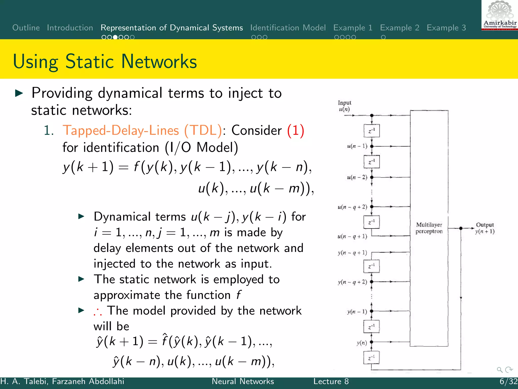
1. Using Static Networks: Providing the
dynamics out of the network and apply static
networks such as multilayer networks (MLN).
Consists of an input layer, output layer
and at least one hidden layer
In fig. there are two hidden layers with
three weight matrices W1, W2 and W3
and a diagonal nonlinear operator Γ with
activation function elements.
Each layer of the network can be
represented by Ni [u] = Γ[Wi u].
The I/O mapping of MLN can be
represented by y = N[u] =
Γ[W3Γ[W2Γ[W1u]]] = N3N2N1[u]
The weights Wi are adjusted s.t min a
function of the error between the
network output y and desired output yd .
H. A. Talebi, Farzaneh Abdollahi Neural Networks Lecture 8 4/32
5. Outline Introduction Representation of Dynamical Systems Identification Model Example 1 Example 2 Example 3
Using Static Networks
The universal approximation theorem shows that a three layers NN with a
backpropagation training algorithm has the potential of behaving as a
universal approximator
Universal Approximation Theorem: Given any > 0 and any L2
function f : [0, 1]n ∈ Rn → Rm, there exists a three-layer
backpropagation network that can approximate f within mean-square
error accuracy.
H. A. Talebi, Farzaneh Abdollahi Neural Networks Lecture 8 5/32
6. Outline Introduction Representation of Dynamical Systems Identification Model Example 1 Example 2 Example 3
Using Static Networks
Providing dynamical terms to inject to
static networks:
1. Tapped-Delay-Lines (TDL): Consider (1)
for identification (I/O Model)
y(k + 1) = f (y(k), y(k − 1), ..., y(k − n),
u(k), ..., u(k − m)),
Dynamical terms u(k − j), y(k − i) for
i = 1, ..., n, j = 1, ..., m is made by
delay elements out of the network and
injected to the network as input.
The static network is employed to
approximate the function f
∴ The model provided by the network
will be
ˆy(k + 1) = ˆf (ˆy(k), ˆy(k − 1), ...,
ˆy(k − n), u(k), ..., u(k − m)),
H. A. Talebi, Farzaneh Abdollahi Neural Networks Lecture 8 6/32
7. Outline Introduction Representation of Dynamical Systems Identification Model Example 1 Example 2 Example 3
Using Static Networks
Considering State Space model:
x(k + 1) = f (x(k), x(k − 1), ..., x(k − n), u(k), ..., u(k − m)),
y(k) = Cx(k)
H. A. Talebi, Farzaneh Abdollahi Neural Networks Lecture 8 7/32
8. Outline Introduction Representation of Dynamical Systems Identification Model Example 1 Example 2 Example 3
Using Static Networks
2 Filtering
in continuous-time networks the
delay operator can be shown by
integrator.
The dynamical model can be
represented by an MLN , N1[.], + a
transfer matrix of linear function,
W (s).
For example:
˙x(t) = f (x, u)±Ax,
where A is Hurwitz. Define
g(x, u) = f (x, u) − Ax
˙x = g(x, u) + Ax
Fig, shows 4 configurations using
filter.
H. A. Talebi, Farzaneh Abdollahi Neural Networks Lecture 8 8/32
9. Outline Introduction Representation of Dynamical Systems Identification Model Example 1 Example 2 Example 3
Representation of Dynamical Systems by Neural Networks
2. Using Dynamic Networks: Time-Delay
Neural Networks (TDNN) [?] , Recurrent
networks such as Hopfield:
Consists of a single layer network N1,
included in feedback configuration and a
time delay
Can represent discrete-time dynamical
system as :
x(k + 1) = N1[x(k)], x(0) = x0
If N1 is suitably chosen, the solution of the
NN converge to the same equilibrium
point of the system.
In continuous-time, the feedback path has
a diagonal transfer matrix with 1/(s − α)
in diagonal.
∴ the system is represented by
˙x = αx + N1[x] + I
H. A. Talebi, Farzaneh Abdollahi Neural Networks Lecture 8 9/32
10. Outline Introduction Representation of Dynamical Systems Identification Model Example 1 Example 2 Example 3
Neural Networks Identification Model
Two principles of identification problems:
1. Identification model
2. Method of adjusting its parameters based on
identification error e(t)
Identification Model
1. Direct modeling:
it is applicable for control, monitoring,
simulation, signal processing
The objective: output of NN ˆy converge to
output of the system y(k)
∴ the signal of target is output of the system
Identification error e = y(k) − ˆy(k) can be
used for training.
The NN can be a MLN training with BP, such
that minimizes the identification error.
The structure of identification shown in Fig
named Parallel Model
H. A. Talebi, Farzaneh Abdollahi Neural Networks Lecture 8 10/32
11. Outline Introduction Representation of Dynamical Systems Identification Model Example 1 Example 2 Example 3
Direct Modeling
Drawback of parallel model:
There is a feedback in this
model which some times
makes convergence difficult
or even impossible.
2. Series-Parallel Model
In this model the
output of system is
fed to the NN
H. A. Talebi, Farzaneh Abdollahi Neural Networks Lecture 8 11/32
12. Outline Introduction Representation of Dynamical Systems Identification Model Example 1 Example 2 Example 3
Inverse Modeling
It is employed for the control
techniques which require inverse
dynamic
Objective is finding f −1, i.e.,
y → u
Input of the plant is target, u
Error identification is defined
e = u − ˆu
H. A. Talebi, Farzaneh Abdollahi Neural Networks Lecture 8 12/32
13. Outline Introduction Representation of Dynamical Systems Identification Model Example 1 Example 2 Example 3
Example 1: Using Filtering
Consider the nonlinear system
˙x = f (x, u) (2)
u ∈ Rm
: input vector, x ∈ Rn
: state vector, f (.): an unknown function.
Open loop system is stable.
Objective: Identifying f
Define filter:
Adding Ax to and subtracting from (2), where A is an arbitrary Hurwitz
matrix ˙x = Ax + g(x, u) (3)
where g(x, u) = f (x, u) − Ax.
Corresponding to the Hurwitz matrix A, M(s) := (sI − A)−1
is an n × n matrix
whose elements are stable transfer functions.
H. A. Talebi, Farzaneh Abdollahi Neural Networks Lecture 8 13/32
14. Outline Introduction Representation of Dynamical Systems Identification Model Example 1 Example 2 Example 3
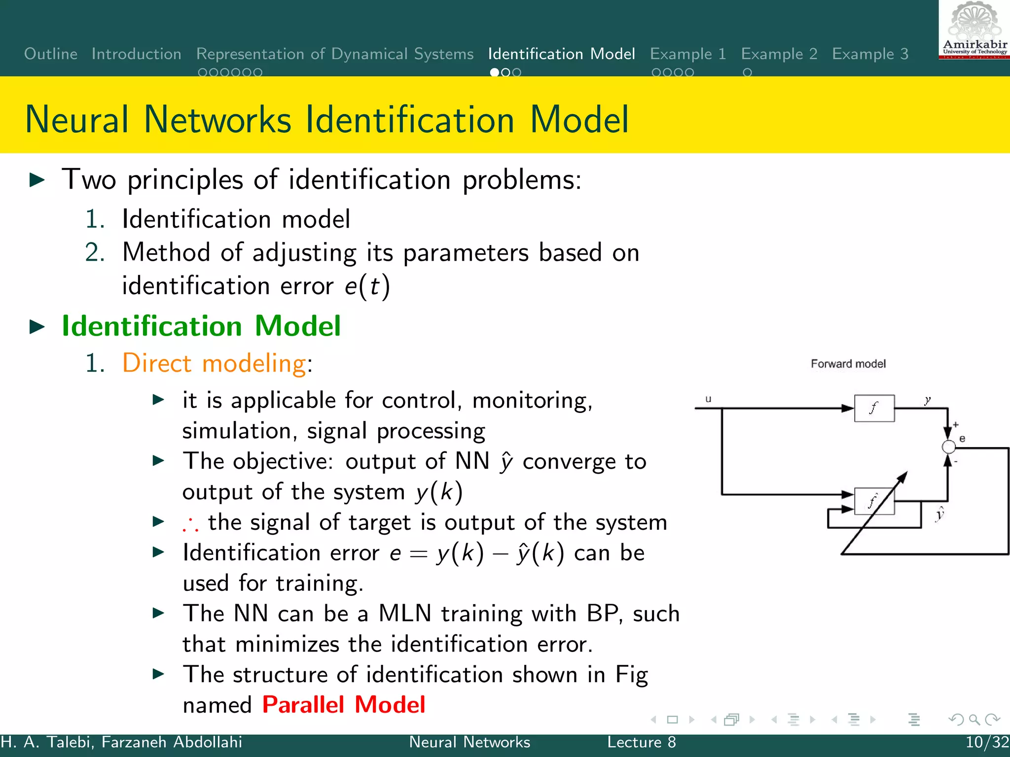
The model for identification purposes:
˙ˆx = Aˆx + ˆg(ˆx, u)
The identification scheme is based on the parallel configuration
The states of the model are fed to the input of the neural network.
an MLP with at least three layers can represent the nonlinear function g as:
g(x, u) = W σ(V ¯x)
W and V are the ideal but unknown weight matrices
¯x = [x u]T
,
σ(.) is the transfer function of the hidden neurons that is usually considered
as a sigmoidal function:
σi (Vi ¯x) =
2
1 + exp−2Vi ¯x
− 1
where Vi is the ith row of V,
σi (Vi ¯x) is the ith element of σ(V ¯x).
H. A. Talebi, Farzaneh Abdollahi Neural Networks Lecture 8 14/32
15. Outline Introduction Representation of Dynamical Systems Identification Model Example 1 Example 2 Example 3
g can be approximated by NN as
ˆg(ˆx, u) = ˆW σ( ˆV ˆ¯x)
The identifier is then given by
˙ˆx(t) = Aˆx + ˆW σ( ˆV ˆ¯x) + (x)
(x) ≤ N is the neural network’s bounded approximation error
the error dynamics:
˙˜x(t) = A˜x + ˜W σ( ˆV ˆ¯x) + w(t)
˜x = x − ˆx: identification error
˜W = W − ˆW , w(t) = W [σ(V ¯x) − σ( ˆV ˆ¯x)] − (x) is a bounded
disturbance term, i.e, w(t) ≤ ¯w for some pos. const. ¯w, due to the
sigmoidal function.
Objective function J = 1
2(˜xT ˜x)
H. A. Talebi, Farzaneh Abdollahi Neural Networks Lecture 8 15/32
16. Outline Introduction Representation of Dynamical Systems Identification Model Example 1 Example 2 Example 3
Training:
Updating weights:
˙ˆW = −η1(
∂J
∂ ˆW
) − ρ1 ˜x ˆW
˙ˆV = −η2(
∂J
∂ ˆV
) − ρ2 ˜x ˆV
Therefore:
netˆv = ˆV ˆ¯x
netˆw = ˆW σ( ˆV ˆ¯x).
∂J
∂ ˆW
and ∂J
∂ ˆV
can be computed according to
∂J
∂ ˆW
=
∂J
∂netˆw
.
∂netˆw
∂ ˆW
∂J
∂ ˆV
=
∂J
∂netˆv
.
∂netˆv
∂ ˆV
H. A. Talebi, Farzaneh Abdollahi Neural Networks Lecture 8 16/32
17. Outline Introduction Representation of Dynamical Systems Identification Model Example 1 Example 2 Example 3
∂J
∂netˆw
=
∂J
∂˜x
.
∂˜x
∂ˆx
.
∂ˆx
∂netˆw
= −˜xT
.
∂ˆx
∂netˆw
∂J
∂netˆv
=
∂J
∂˜x
.
∂˜x
∂ˆx
.
∂ˆx
∂netˆv
= −˜xT
.
∂ˆx
∂netˆv
and
∂netˆw
∂ ˆW
= σ( ˆV ˆ¯x)
∂netˆv
∂ ˆV
= ˆ¯x
∂ ˙ˆx(t)
∂netˆw
= A
∂ˆx
∂netˆw
+
∂ˆg
∂netˆw
∂ ˙ˆx(t)
∂netˆv
= A
∂ˆx
∂netˆv
+
∂ˆg
∂netˆv
.
Which is dynamic BP. Modify BP algorithm s.t. the static
approximations of ∂ˆx
∂netˆw
and ∂ˆx
∂netˆv
(˙ˆx = 0)
H. A. Talebi, Farzaneh Abdollahi Neural Networks Lecture 8 17/32
18. Outline Introduction Representation of Dynamical Systems Identification Model Example 1 Example 2 Example 3
Thus, ∂ˆx
∂netˆw
= −A−1
∂ˆx
∂netˆv
= −A−1 ˆW (I − Λ( ˆV ˆ¯x))
where
Λ( ˆV ˆ¯x) = diag{σ2
i ( ˆVi ˆ¯x)}, i = 1, 2, ..., m.
Finally
˙ˆW = −η1(˜xT
A−1
)T
(σ( ˆV ˆ¯x))T
− ρ1 ˜x ˆW
˙ˆV = −η2(˜xT
A−1 ˆW (I − Λ( ˆV ˆ¯x)))T ˆ¯xT
− ρ2 ˜x ˆV
˜W = W − ˆW and ˜V = V − ˆV ,
It can be shown that ˜x, ˜W , and ˜V ∈ L∞
The estimation error and the weights error are all ultimately bounded [?].
H. A. Talebi, Farzaneh Abdollahi Neural Networks Lecture 8 18/32
19. Outline Introduction Representation of Dynamical Systems Identification Model Example 1 Example 2 Example 3
Series-Parallel Identifier
The function g can be approximated
byˆg(x, u) = ˆW σ( ˆV ¯x)
Only ˆ¯x is changed to ¯x.
The error dynamics
˙˜x(t) = A˜x + ˜W σ( ˆV ¯x) + w(t) where
w(t) = W [σ(V ¯x) − σ( ˆV ¯x)] + (x)
only definition of w(t) is changed.
Applying this change, the rest remains
the same
H. A. Talebi, Farzaneh Abdollahi Neural Networks Lecture 8 19/32
20. Outline Introduction Representation of Dynamical Systems Identification Model Example 1 Example 2 Example 3
Using Dynamic BP Without Static Approximation
∂J
∂ ˆW
=
∂J
∂˜x
.
∂˜x
∂ˆx
.
∂ˆx
∂netˆw
.
∂netˆw
∂ ˆW
= −˜xT
.
∂ˆx
∂netˆw
.σ( ˆV ˆ¯x)
∂J
∂ ˆV
=
∂J
∂˜x
.
∂˜x
∂ˆx
.
∂ˆx
∂netˆv
.
∂netˆv
∂ ˆV
= −˜xT
.
∂ˆx
∂netˆv
ˆ¯x
and dw =
∂ˆx(t)
∂netˆw
˙dw =
∂ ˙ˆx(t)
∂netˆw
= Adw +
∂ˆg
∂netˆw
= Adw + 1 (4)
dv =
∂ˆx(t)
∂netˆv
˙dv =
∂ ˙ˆx(t)
∂netˆv
= Adv +
∂ˆg
∂netˆv
= Adv + ˆW (I − Λ( ˆV ˆ¯x)) (5)
H. A. Talebi, Farzaneh Abdollahi Neural Networks Lecture 8 20/32
21. Outline Introduction Representation of Dynamical Systems Identification Model Example 1 Example 2 Example 3
Using Dynamic BP Without Static Approximation
Finally
˙ˆW = η1(˜xT
dw )T
(σ( ˆV ˆ¯x))T
− ρ1 ˜x ˆW
˙ˆV = η2(˜xT
dv ))T ˆ¯xT
− ρ2 ˜x ˆV
In learning rule procedure, first (4) and (5) should be solved then the
weights W and V is updated
H. A. Talebi, Farzaneh Abdollahi Neural Networks Lecture 8 21/32
22. Outline Introduction Representation of Dynamical Systems Identification Model Example 1 Example 2 Example 3
Case Study: Simulation Results on SSRMS
The Space Station Remote Manipulator System (SSRMS) is a 7 DoF
robot which has 7 revolute joints and two long flexible links (booms).
The SSRMS have no uniform mass and stiffness distributions. Most of its
masses are concentrated at the joints, and the joint structural flexibilities
contribute a major portion of the overall arm flexibility.
Dynamics of a flexible–link manipulator
M(q)¨q + h(q, ˙q) + Kq + F ˙q = u
u = [τT
01×m]T
, q = [θT
δT
]T
,
θ is the n × 1 vector of joint variables
δ is the m × 1 vector of deflection variables
h = [h1(q, ˙q) h2(q, ˙q)]T
: including gravity, Coriolis, and centrifugal forces;
M is the mass matrix,
K =
0n×n 0n×m
0m×n Km×m
is the stiffness matrix,
F = diag{F1, F2}: the viscous friction at the hub and in the structure,
τ: input torque.
H. A. Talebi, Farzaneh Abdollahi Neural Networks Lecture 8 22/32
23. Outline Introduction Representation of Dynamical Systems Identification Model Example 1 Example 2 Example 3
Case Study: Simulation Results on SSRMS
http://english.sohu.com/20050729/n226492517.shtml
H. A. Talebi, Farzaneh Abdollahi Neural Networks Lecture 8 23/32
24. Outline Introduction Representation of Dynamical Systems Identification Model Example 1 Example 2 Example 3
Case Study: Simulation Results on SSRMS
A joint PD control is applied to stabilize the closed-loop system
boundedness of the signal x(t) is assured.
For a two link flexible manipulator
x = [θ1... θ7
˙θ1... ˙θ7 δ11 δ12 δ21 δ22
˙δ11
˙δ12
˙δ21
˙δ22]T
The input: u = [τ1, ..., τ7]
A is defined as A = −2I ∈ R22×22
Reference trajectory: sin(t)
The identifier:
Series-parallel
A three-layer NN network: 29 neurons in the input layer, 20 neurons in the
hidden layer, and 22 neurons in the output layer.
The 22 outputs correspond to
7 joint positions
7 joint velocities
4 in-plane deflection variables
4 out-of plane deflection variables
The learning rates and damping factors: η1 = η2 = 0.1, ρ1 = ρ2 = 0.001.
H. A. Talebi, Farzaneh Abdollahi Neural Networks Lecture 8 24/32
25. Outline Introduction Representation of Dynamical Systems Identification Model Example 1 Example 2 Example 3
Case Study: Simulation Results on SSRMS
Simulation results for the SSRMS: (a-g) The joint positions, and (h-n)
the joint velocities.
H. A. Talebi, Farzaneh Abdollahi Neural Networks Lecture 8 25/32
26. Outline Introduction Representation of Dynamical Systems Identification Model Example 1 Example 2 Example 3
Example 2: TDL
Consider the following nonlinear
system
y(k) = f (y(k − 1), ..., y(k − n))
+b0u(k) + ... + bmu(k − m)
u: input, y:output, f (.): an
unknown function.
Open loop system is stable.
Objective: Identifying f
Series-parallel identifier is applied.
β = [b0, b1, ..., bm]
Cost function: J = 1
2 e2
i where
ei = y − yh,
H. A. Talebi, Farzaneh Abdollahi Neural Networks Lecture 8 26/32
27. Outline Introduction Representation of Dynamical Systems Identification Model Example 1 Example 2 Example 3
Consider Linear in parameter MLP,
In sigmoidal function.σ, the weights of first layer is fixed V = I:
σi (¯x) = 2
1+exp−2¯x − 1
Updating law: w = −η( ∂J
∂w )
∴ ∂J
∂w = ∂J
∂ei
∂ei
∂w = −ei
∂N(.)
∂w
∂N(.)
∂w is obtained by BP method.
Numerical Example: Consider a second order system
yp(k + 1) = f [yp(k), yp(k − 1)] + u(k)
where f [yp(k), yp(k − 1)] =
yp(k)yp(k−1)[yp(k)+2.5]
1+y2
p (k)+y2
p (k−1)
.
After checking the stability system
Apply series-parallel identifier
u is random signal informally is distributed in [−2, 2]
η = 0.25
H. A. Talebi, Farzaneh Abdollahi Neural Networks Lecture 8 27/32
28. Outline Introduction Representation of Dynamical Systems Identification Model Example 1 Example 2 Example 3
Numerical Example Cont’d
The outputs of the plant and the model after the identification procedure
H. A. Talebi, Farzaneh Abdollahi Neural Networks Lecture 8 28/32
29. Outline Introduction Representation of Dynamical Systems Identification Model Example 1 Example 2 Example 3
Example 3 [?]
A gray box identification,( the system model is known but it includes
some unknown, uncertain and/or time-varying parameters) is
proposed using Hopfield networks
Consider
˙x = A(x, u(t))(θn + θ(t))
y = x
y is the output,
θ is the unknowntime-dependantdeviation from the nominal values
A is a matrix that depends on the input u and the state x
y and A are assumed to be physically measurable.
Objective: estimating θ (i.e. min the estimation error: ˜θ = θ − ˆθ).
H. A. Talebi, Farzaneh Abdollahi Neural Networks Lecture 8 29/32
30. Outline Introduction Representation of Dynamical Systems Identification Model Example 1 Example 2 Example 3
At each time interval assume time
is frozen so that
Ac = A(x(t), u(t)), yc = y(t)
Recall Gradient-Type Hopefield
C du
dt = Wv(t) + I
the weight matrix and the bias
vector are defined:
W = −AT
c Ac, I = AT
c Acθn −AT
c yc
The convergence of the identifier is
proven using Lyapunov method
It is examined for an idealized
single link manipulator
¨x = −g
l sinx − v
ml2 ˙x + 1
ml2 u
assume A = (sinx, ˙x, u) and
θn + θ = (−g
l , − v
ml2 , 1
ml2 )
H. A. Talebi, Farzaneh Abdollahi Neural Networks Lecture 8 30/32
31. Outline Introduction Representation of Dynamical Systems Identification Model Example 1 Example 2 Example 3
H. A. Talebi, Farzaneh Abdollahi Neural Networks Lecture 8 31/32
32. Outline Introduction Representation of Dynamical Systems Identification Model Example 1 Example 2 Example 3
References
K.S. Narendra and K. Parthasarathy, “Identification and control of dynamical systems
using neural networks,” IEEE Trans. on Neural Networks, vol. 1, no. 1, pp. 4–27, March
1990.
H. A. Talebi, Farzaneh Abdollahi Neural Networks Lecture 8 32/32