Downloaded 148 times
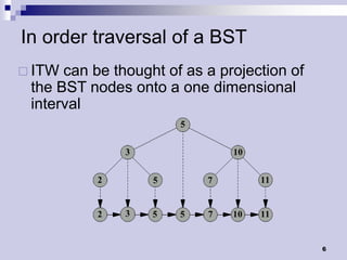
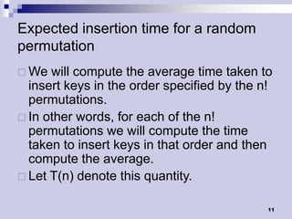
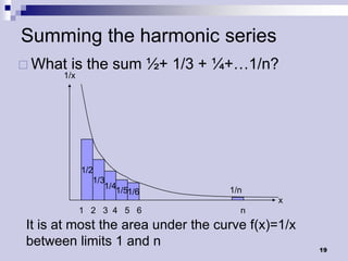
![Deletion Case 2
Ifx has exactly one child, then to delete
x, simply make p[x] point to that child
3](https://image.slidesharecdn.com/lec9-101217101349-phpapp02/85/Lec9-3-320.jpg)
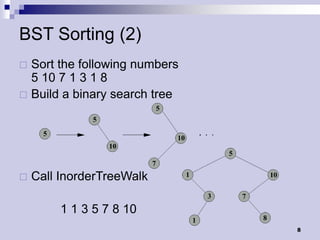
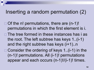
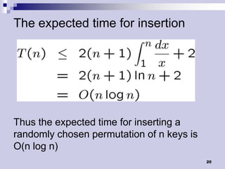
![Delete Pseudocode
TreeDelete(T,z)
01 if left[z] NIL or right[z] = NIL
02 then y z
03 else y TreeSuccessor(z)
04 if left[y] NIL
05 then x left[y]
06 else x right[y]
07 if x NIL
08 then p[x] p[y]
09 if p[y] = NIL
10 then root[T] x
11 else if y = left[p[y]]
12 then left[p[y]] x
13 else right[p[y]] x
14 if y z
15 then key[z] key[y] //copy all fileds of y
16 return y
5](https://image.slidesharecdn.com/lec9-101217101349-phpapp02/85/Lec9-5-320.jpg)
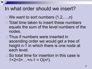
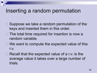
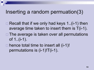
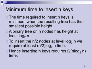
![BST Sorting
Use TreeInsert and InorderTreeWalk to
sort a list of n elements, A
TreeSort(A)
01 root[T] NIL
02 for i 1 to n
03 TreeInsert(T,A[i])
04 InorderTreeWalk(root[T])
7](https://image.slidesharecdn.com/lec9-101217101349-phpapp02/85/Lec9-7-320.jpg)
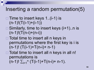
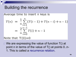
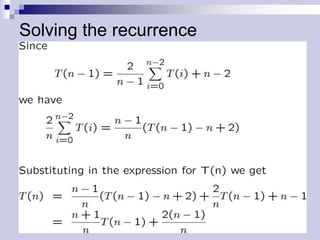

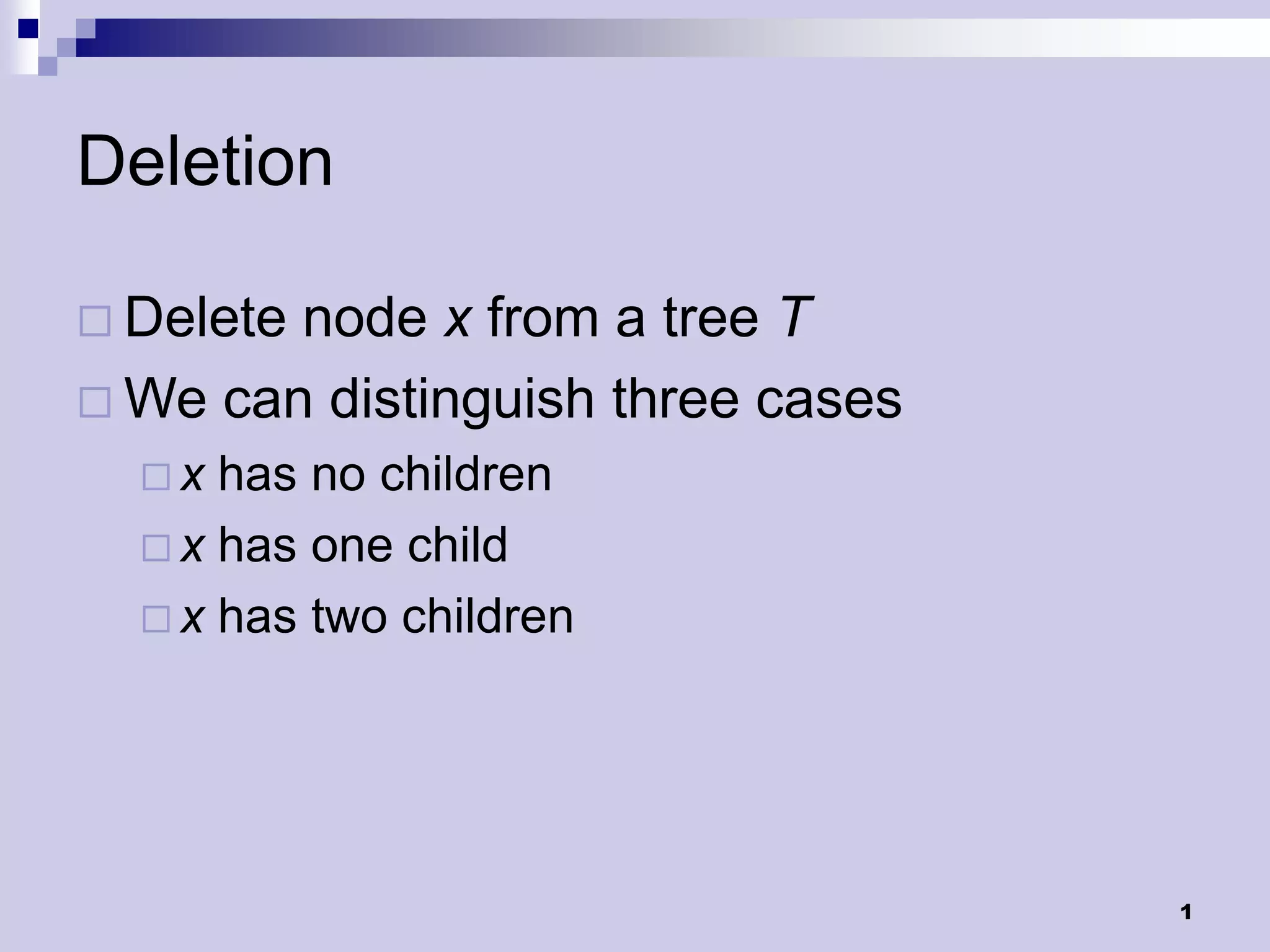
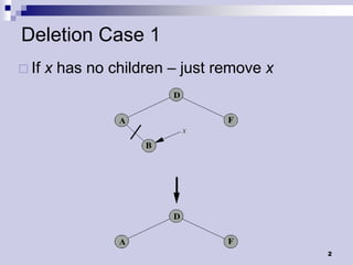
The document discusses three cases for deleting a node from a binary search tree: 1) if the node has no children, simply remove it, 2) if the node has one child, make the parent point to the child, and 3) if the node has two children, find its successor, remove the successor, and replace the node with the successor. It then provides pseudocode for the delete operation and examples of building a BST and performing an in-order traversal.