Download as PDF, PPTX
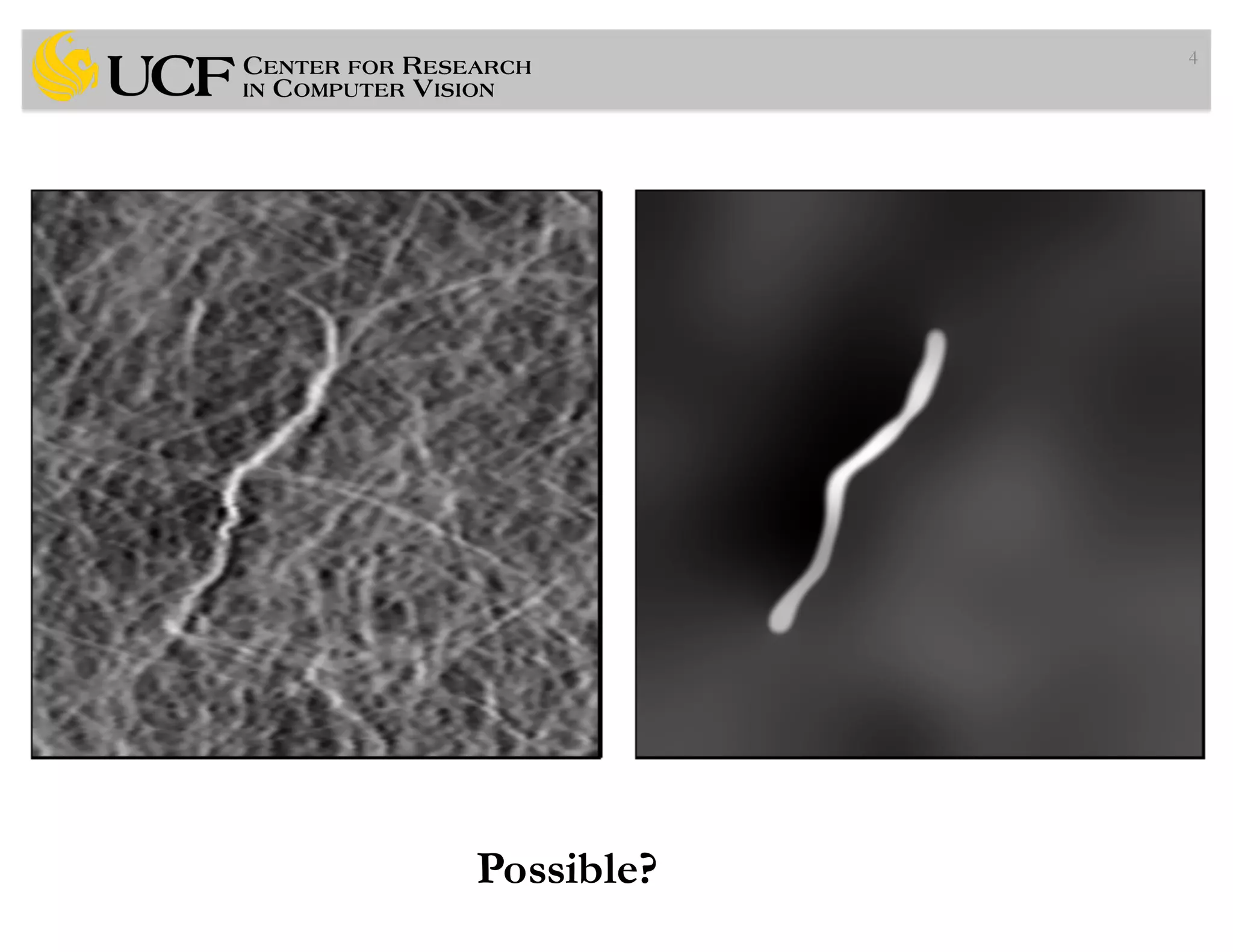
![Perona-Malik (Anisotropic Diffusion) Filtering
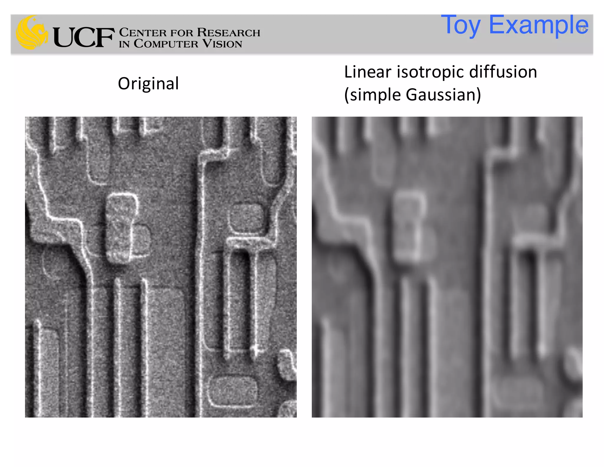
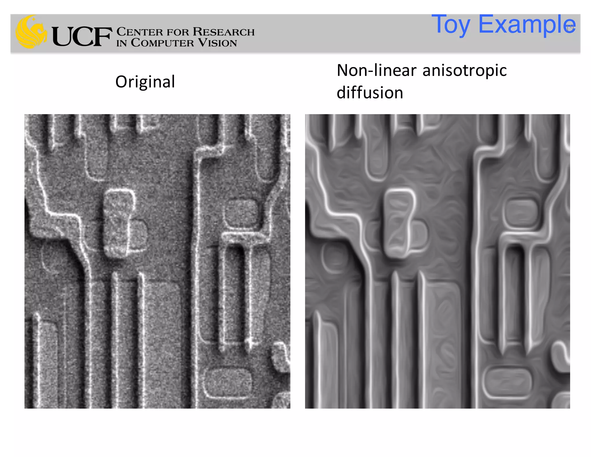
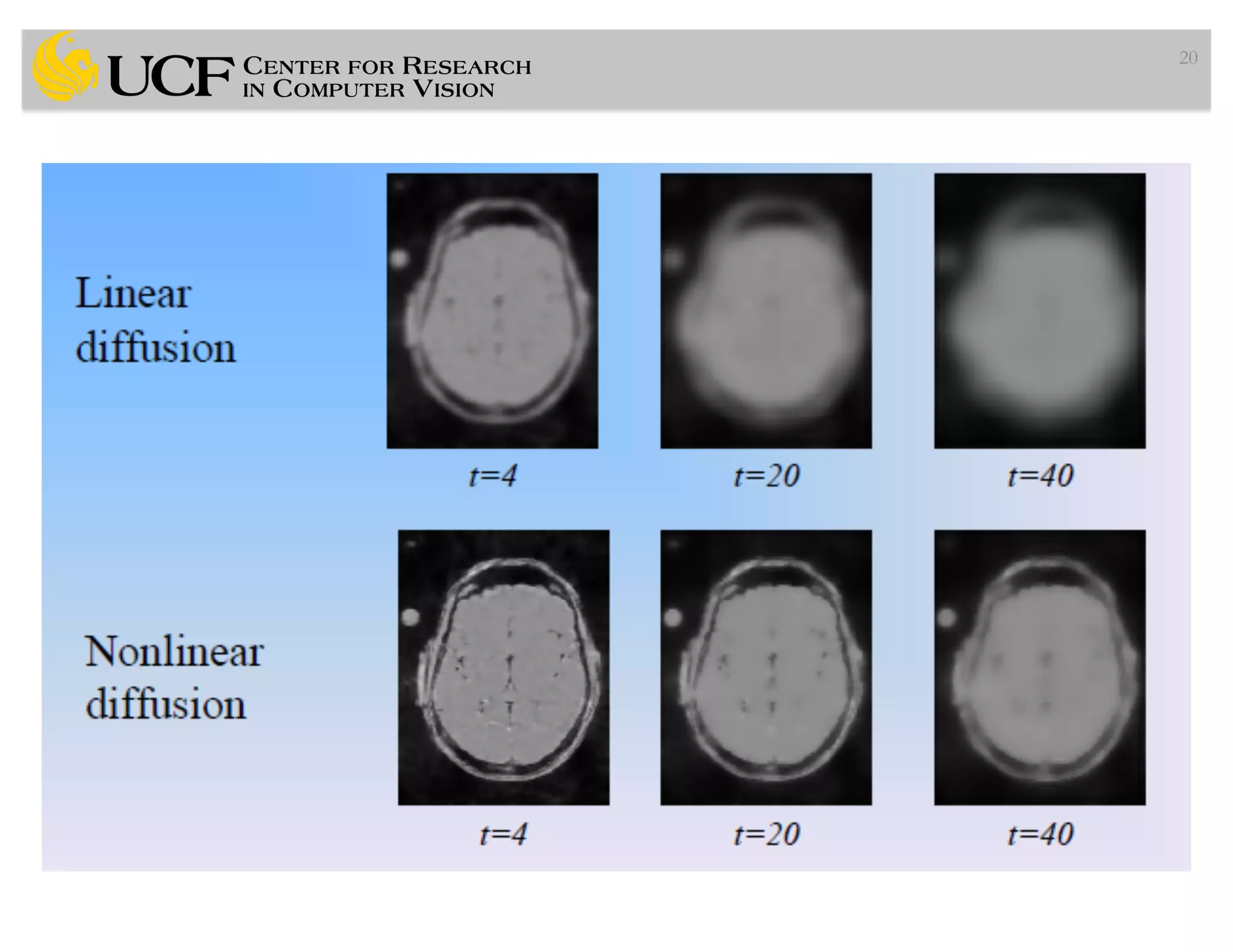
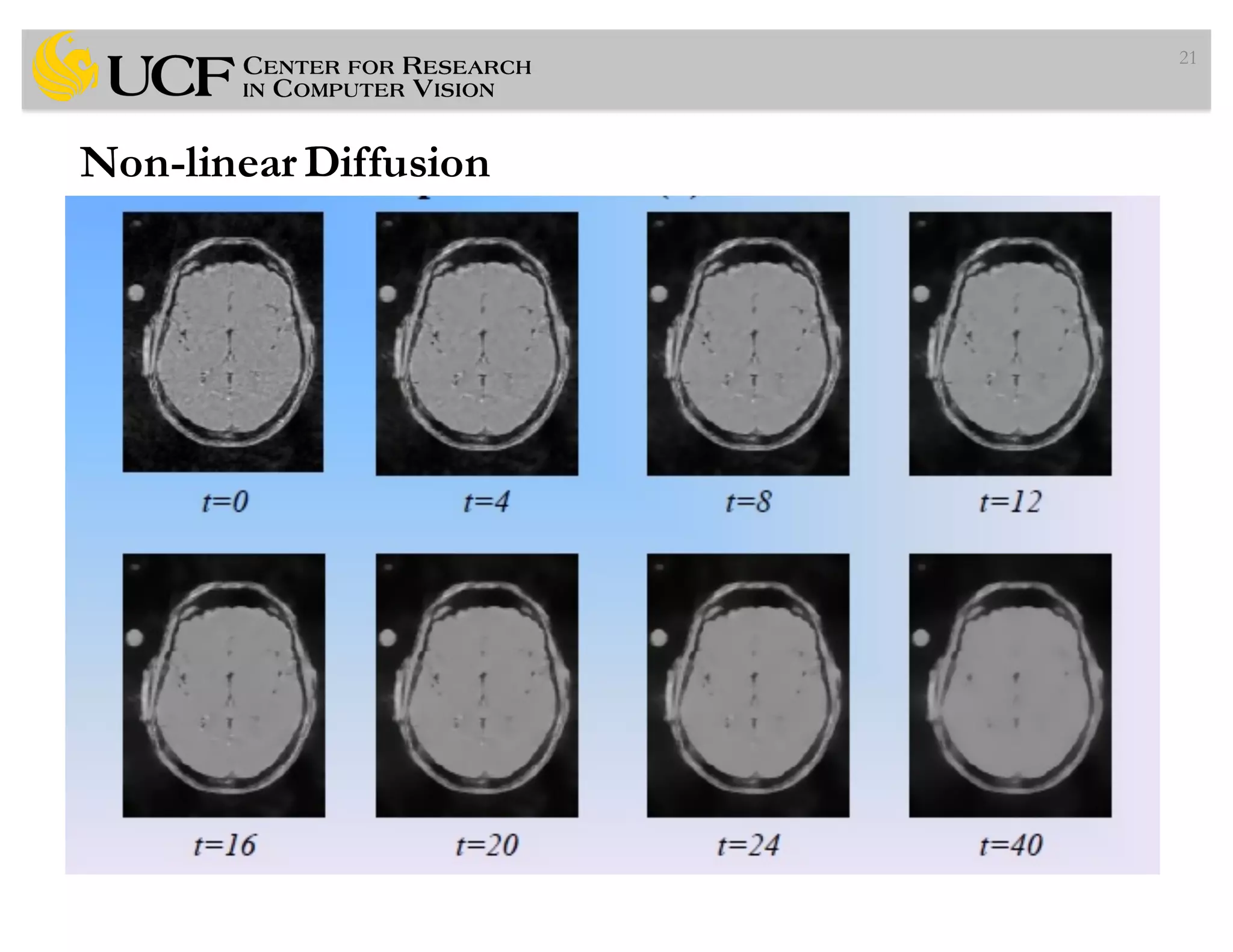
• Perona and Malik propose a nonlinear diffusion method for
avoiding the blurring and localization problems of linear
diffusion filtering [PAMI 1990].
– Smooth the images without removing significant parts of the edges
5](https://image.slidesharecdn.com/lec4-170330052253/75/Lec4-Pre-Processing-Medical-Images-II-5-2048.jpg)
![Perona-Malik (Anisotropic Diffusion) Filtering
• Perona and Malik propose a nonlinear diffusion method for
avoiding the blurring and localization problems of linear
diffusion filtering [PAMI 1990].
– Smooth the images without removing significant parts of the edges
– The smoothing process is considered as diffusion
6](https://image.slidesharecdn.com/lec4-170330052253/75/Lec4-Pre-Processing-Medical-Images-II-6-2048.jpg)
![Perona-Malik (Anisotropic Diffusion) Filtering
• Perona and Malik propose a nonlinear diffusion method for
avoiding the blurring and localization problems of linear
diffusion filtering [PAMI 1990].
– Smooth the images without removing significant parts of the edges
– The smoothing process is considered as diffusion
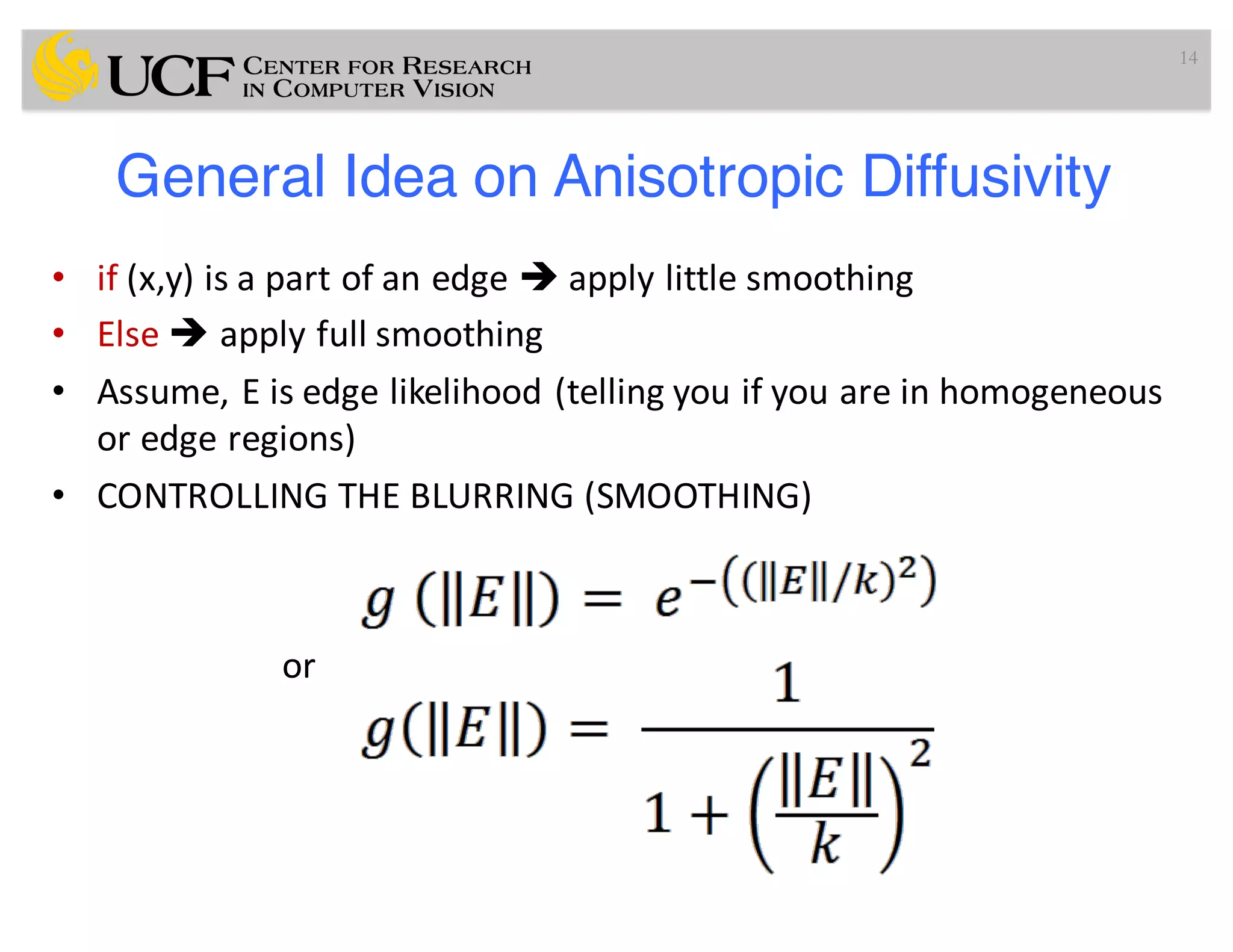
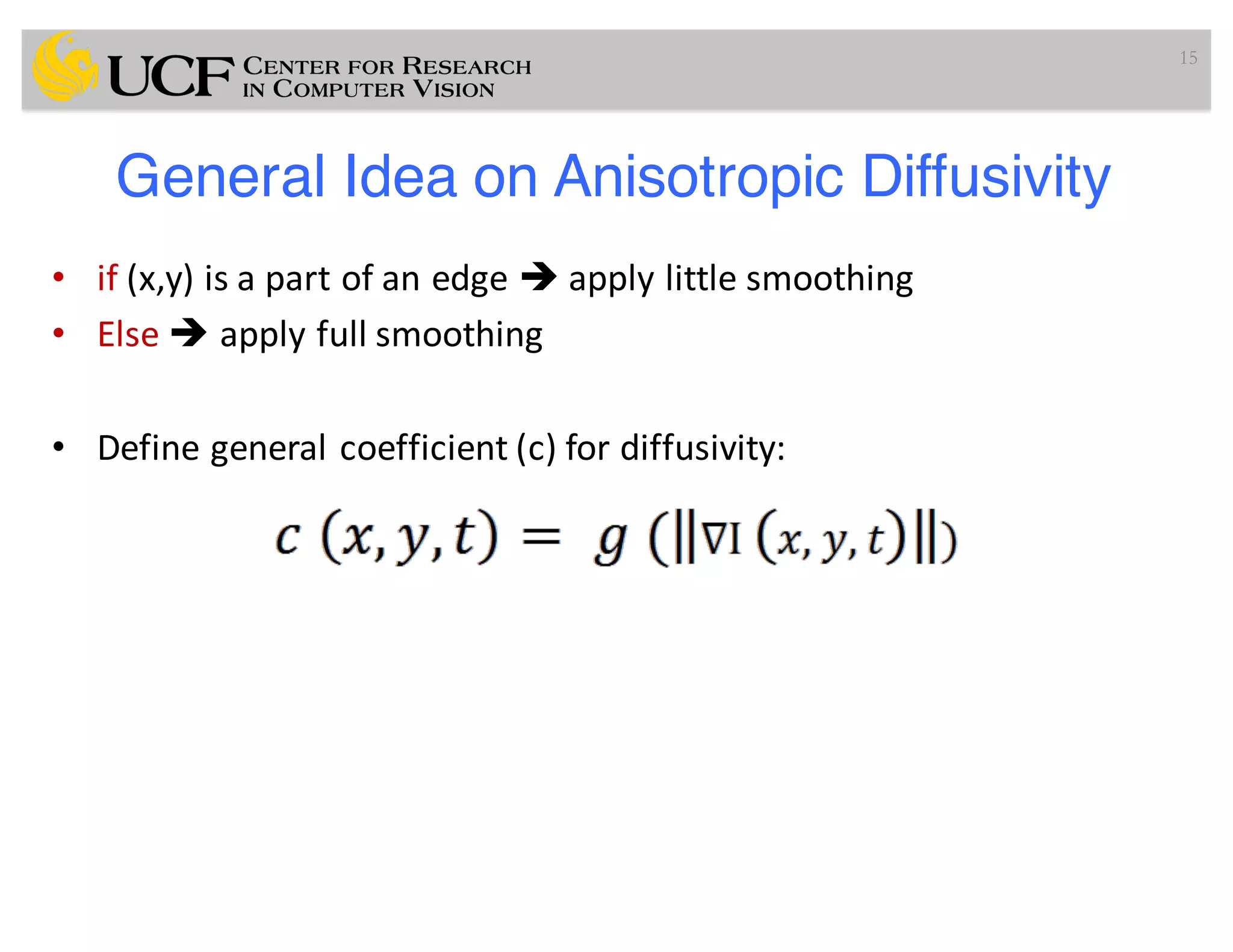
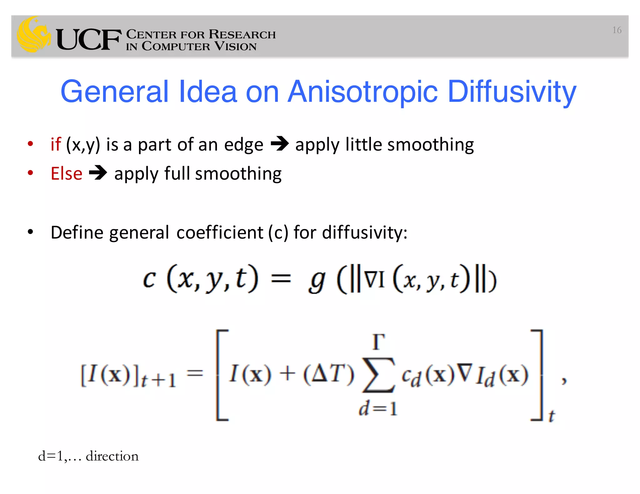
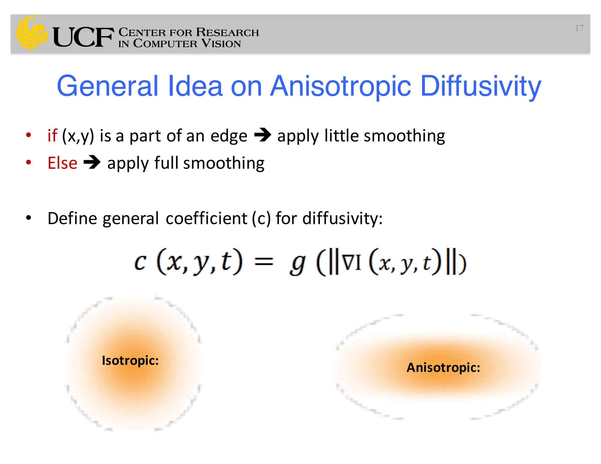
– APPROACH: Increase the diffusivity of filter for large (homogeneous)
regions, and decrease it nearby edges!
7](https://image.slidesharecdn.com/lec4-170330052253/75/Lec4-Pre-Processing-Medical-Images-II-7-2048.jpg)
![Perona-Malik (Anisotropic Diffusion) Filtering
• Perona and Malik propose a nonlinear diffusion method for
avoiding the blurring and localization problems of linear
diffusion filtering [PAMI 1990].
– Smooth the images without removing significant parts of the edges
– The smoothing process is considered as diffusion
– APPROACH: Increase the diffusivity of filter for large (homogeneous)
regions, and decrease it nearby edges!
– How can we understand homogenous and edge regions then?
8](https://image.slidesharecdn.com/lec4-170330052253/75/Lec4-Pre-Processing-Medical-Images-II-8-2048.jpg)
![Perona-Malik (Anisotropic Diffusion) Filtering
• Perona and Malik propose a nonlinear diffusion method for
avoiding the blurring and localization problems of linear
diffusion filtering [PAMI 1990].
– Smooth the images without removing significant parts of the edges
– The smoothing process is considered as diffusion
– APPROACH: Increase the diffusivity of filter for large (homogeneous)
regions, and decrease it nearby edges!
– How can we understand homogenous and edge regions then?
– Edge likelihood (i.e, gradient for instance) can be measured by
9](https://image.slidesharecdn.com/lec4-170330052253/75/Lec4-Pre-Processing-Medical-Images-II-9-2048.jpg)
![Perona-Malik (Anisotropic Diffusion) Filtering
• Perona and Malik propose a nonlinear diffusion method for
avoiding the blurring and localization problems of linear
diffusion filtering [PAMI 1990].
– Smooth the images without removing significant parts of the edges
– The smoothing process is considered as diffusion
– APPROACH: Increase the diffusivity of filter for large (homogeneous)
regions, and decrease it nearby edges!
– How can we understand homogenous and edge regions then?
– Edge likelihood (i.e, gradient for instance) can be measured by
– Perona-Malik filter is based on
10](https://image.slidesharecdn.com/lec4-170330052253/75/Lec4-Pre-Processing-Medical-Images-II-10-2048.jpg)
![Perona-Malik (Anisotropic Diffusion) Filtering
• Perona and Malik propose a nonlinear diffusion method for
avoiding the blurring and localization problems of linear
diffusion filtering [PAMI 1990].
– Smooth the images without removing significant parts of the edges
– The smoothing process is considered as diffusion
– APPROACH: Increase the diffusivity of filter for large (homogeneous)
regions, and decrease it nearby edges!
– How can we understand homogenous and edge regions then?
– Edge likelihood (i.e, gradient for instance) can be measured by
– Perona-Malik filter is based on
where it uses diffusivities such as
11](https://image.slidesharecdn.com/lec4-170330052253/75/Lec4-Pre-Processing-Medical-Images-II-11-2048.jpg)
![Perona-Malik (Anisotropic Diffusion) Filtering
• Perona and Malik propose a nonlinear diffusion method for
avoiding the blurring and localization problems of linear
diffusion filtering [PAMI 1990].
– Smooth the images without removing significant parts of the edges
– The smoothing process is considered as diffusion
– APPROACH: Increase the diffusivity of filter for large (homogeneous)
regions, and decrease it nearby edges!
– How can we understand homogenous and edge regions then?
– Edge likelihood (i.e, gradient for instance) can be measured by
– Perona-Malik filter is based on
where it uses diffusivities such as
– approximation
12](https://image.slidesharecdn.com/lec4-170330052253/75/Lec4-Pre-Processing-Medical-Images-II-12-2048.jpg)

![ITK Implementation of N3
• itkN3MRIBiasFieldCorrectionImageFilterTest
imageDimension
inputImage
outputImage
[shrinkFactor] [maskImage] [numberOfIterations]
[numberOfFittingLevels] [outputBiasField]
55
Input parameters
opt. parameters](https://image.slidesharecdn.com/lec4-170330052253/75/Lec4-Pre-Processing-Medical-Images-II-55-2048.jpg)
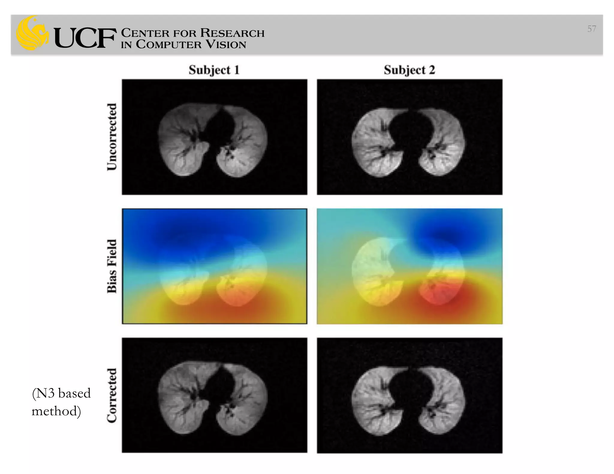
![ITK Implementation of N3
• itkN3MRIBiasFieldCorrectionImageFilterTest
imageDimension
inputImage
outputImage
[shrinkFactor] [maskImage] [numberOfIterations]
[numberOfFittingLevels] [outputBiasField]
56
Input parameters
opt. parameters
itkN3MRIBiasFieldCorrectionImageFilterTest
2 t81slice.nii.gz t81corrected.nii.gz
2 t81mask.nii.gz 50 4 t81biasfield.nii.gz](https://image.slidesharecdn.com/lec4-170330052253/75/Lec4-Pre-Processing-Medical-Images-II-56-2048.jpg)

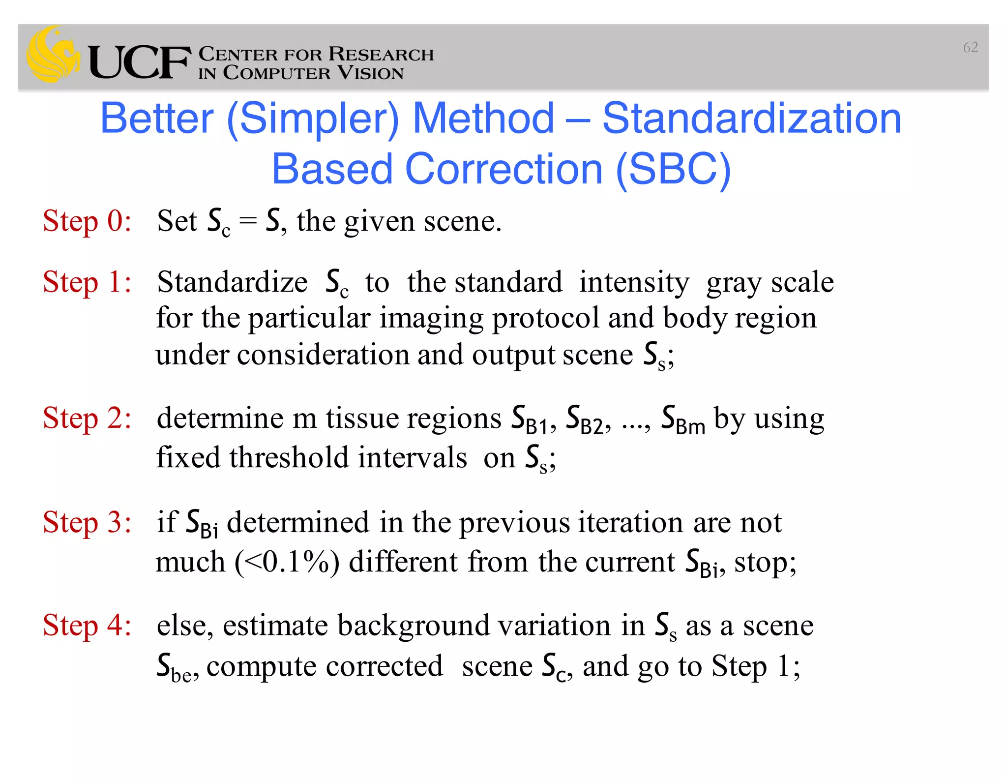
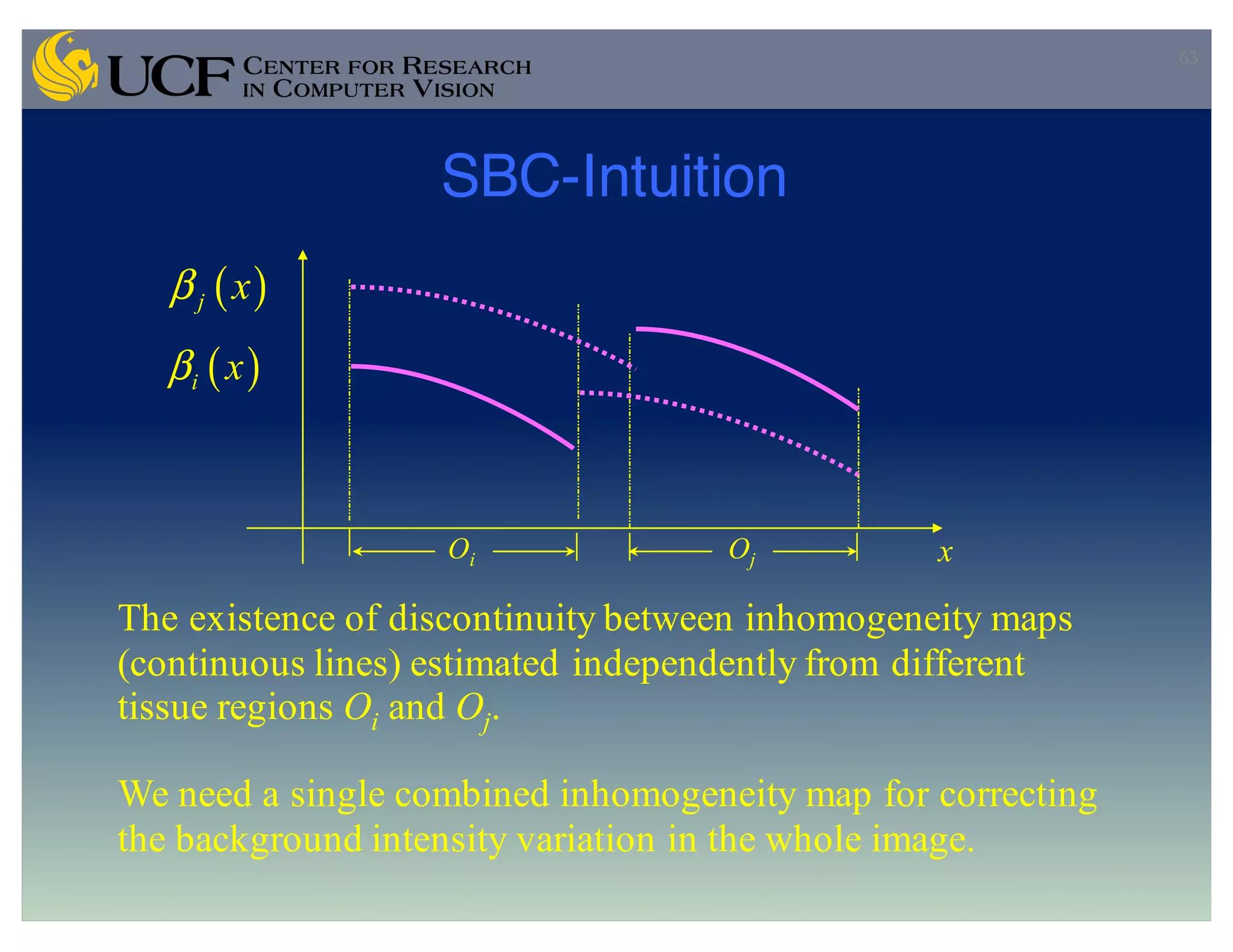
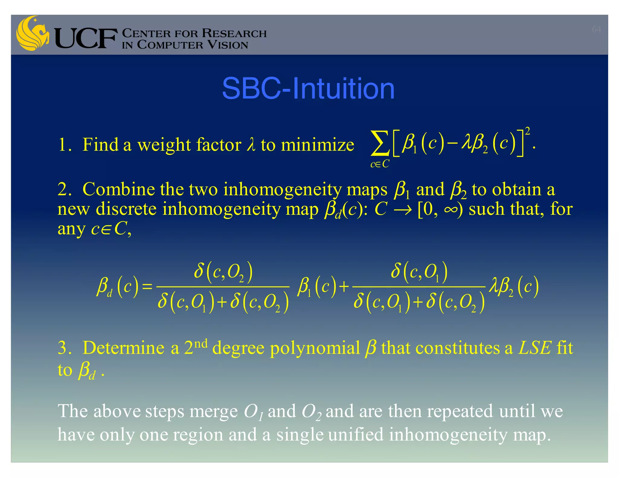
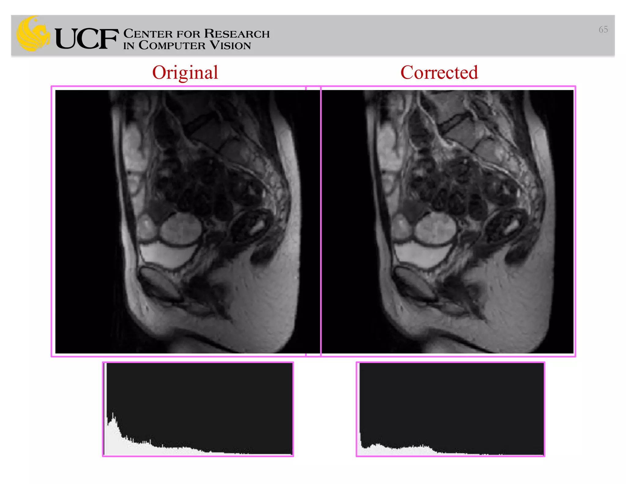
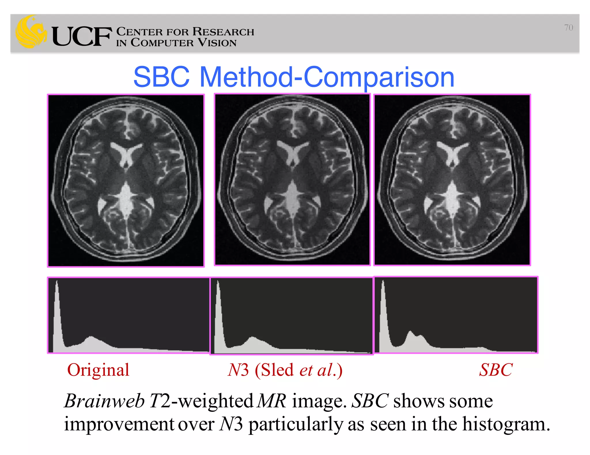
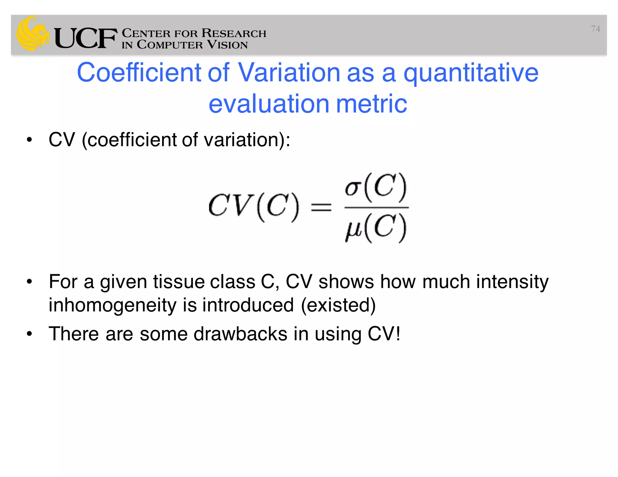
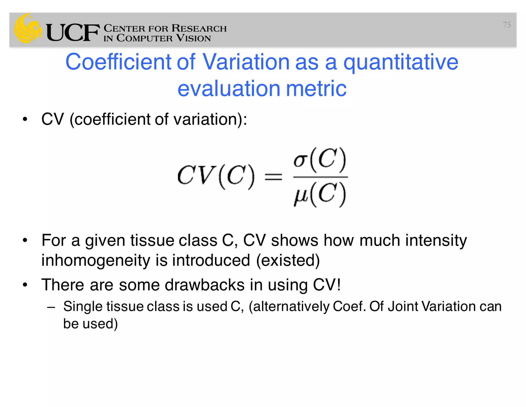
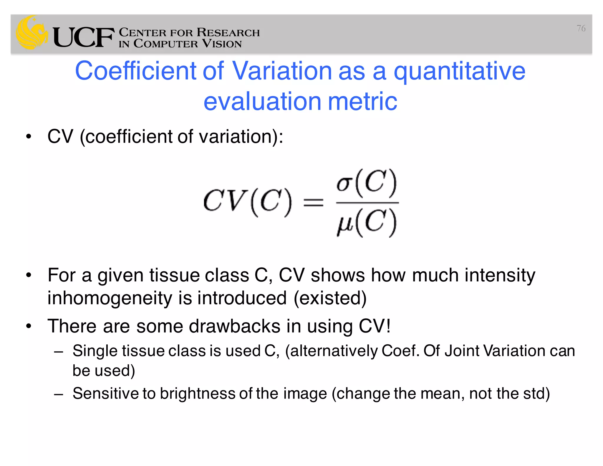

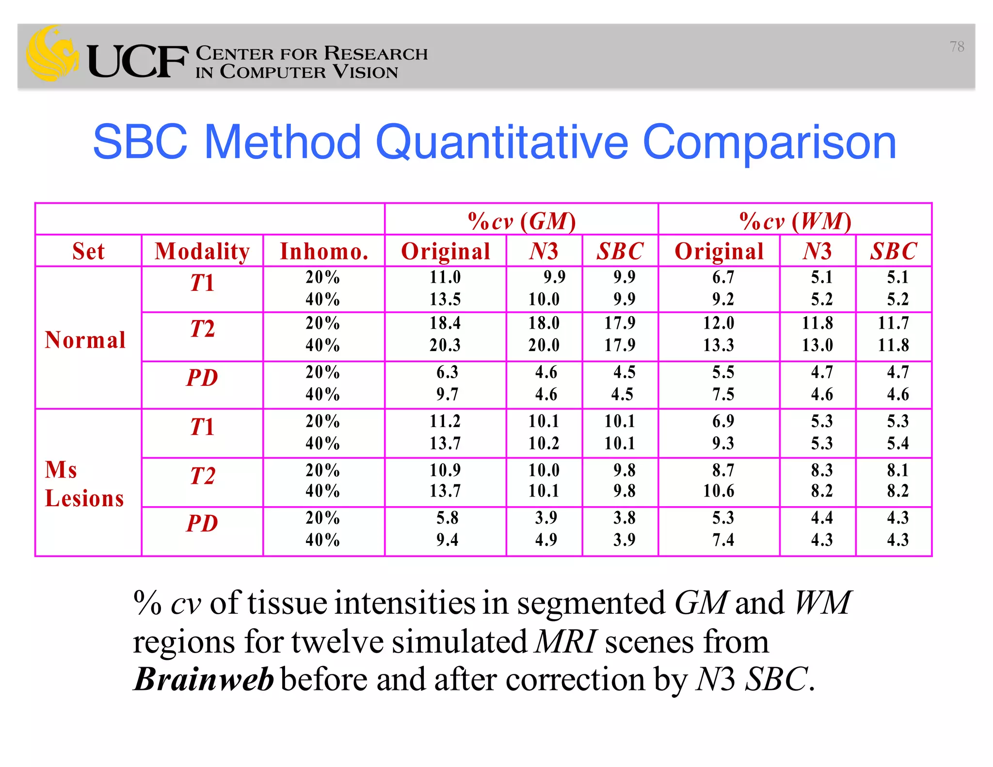
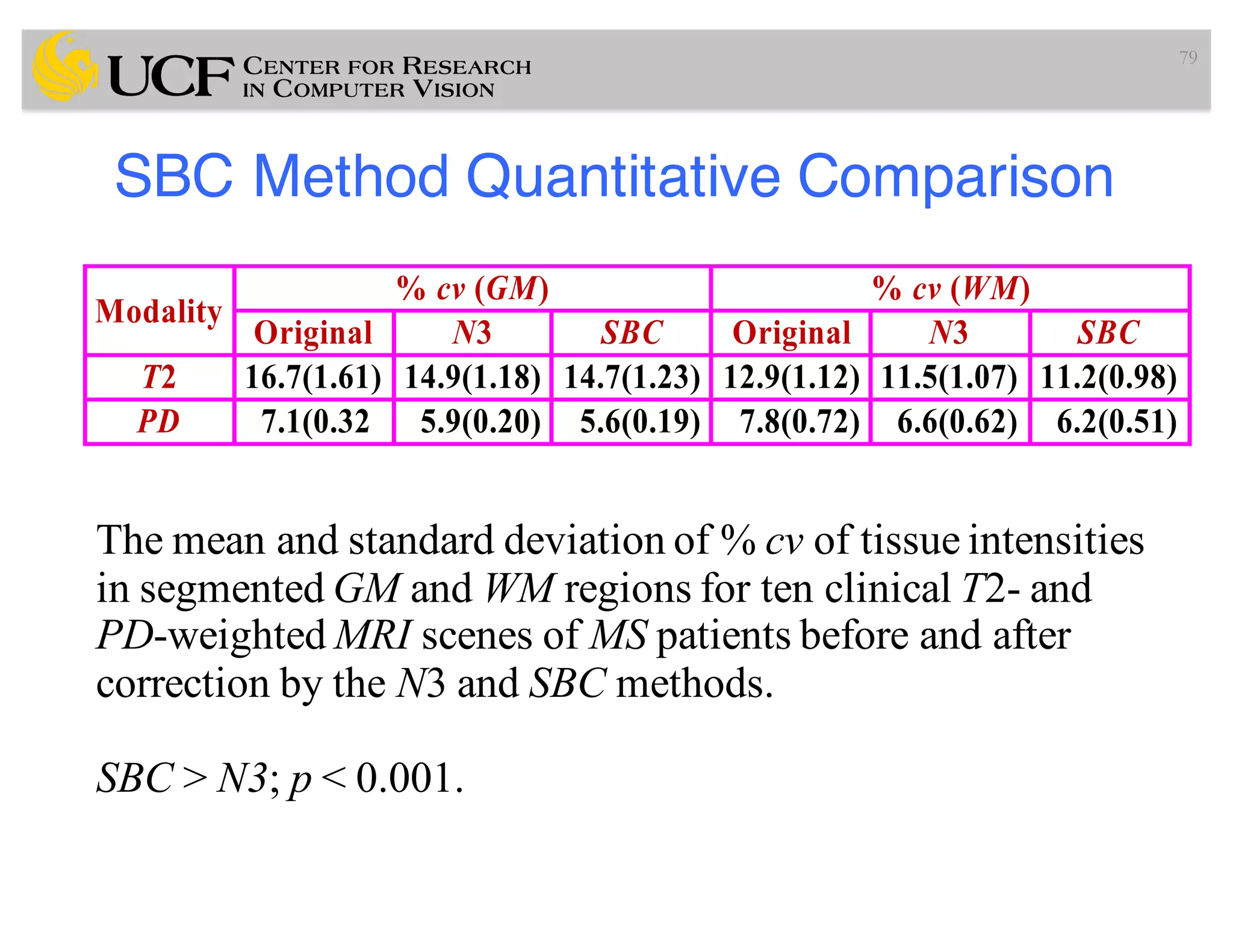

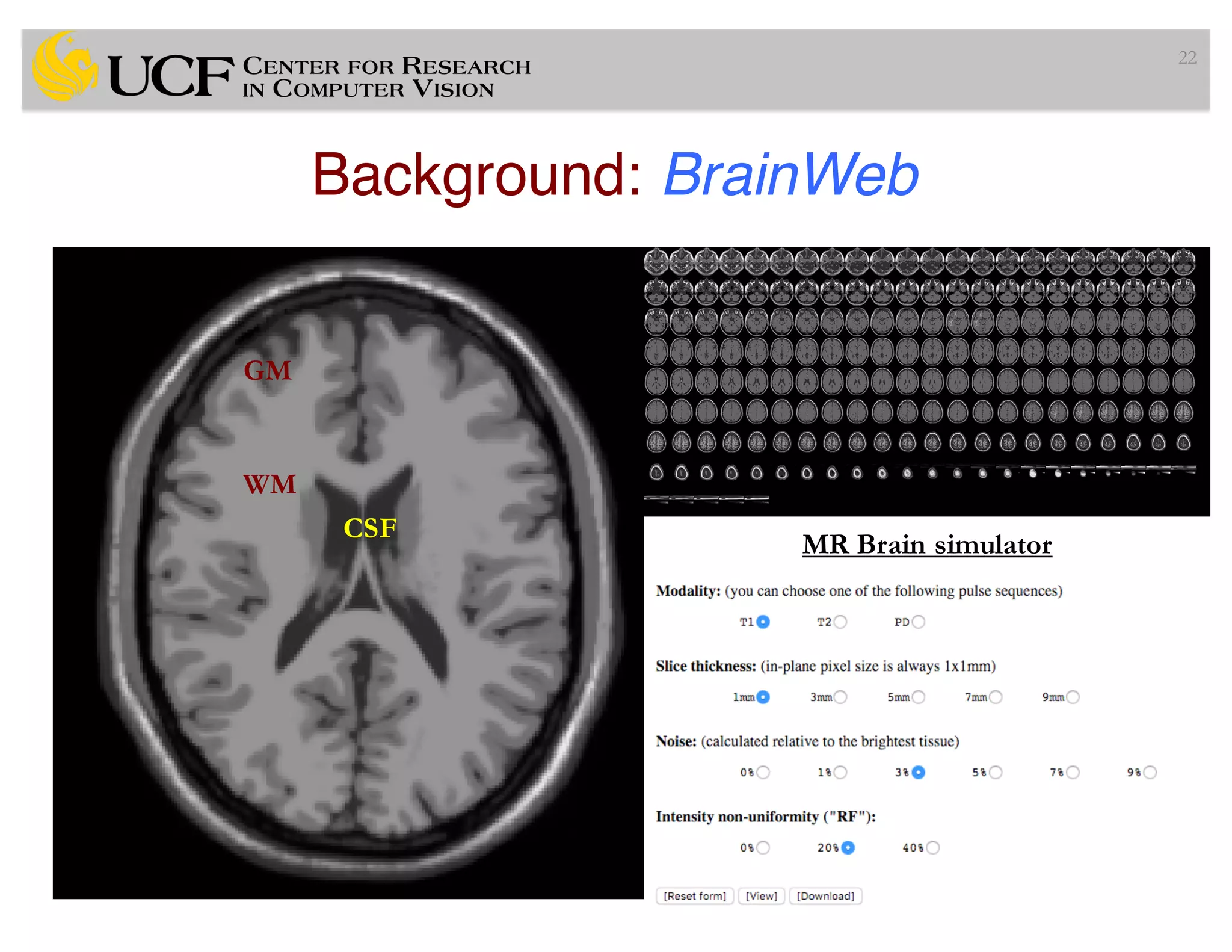
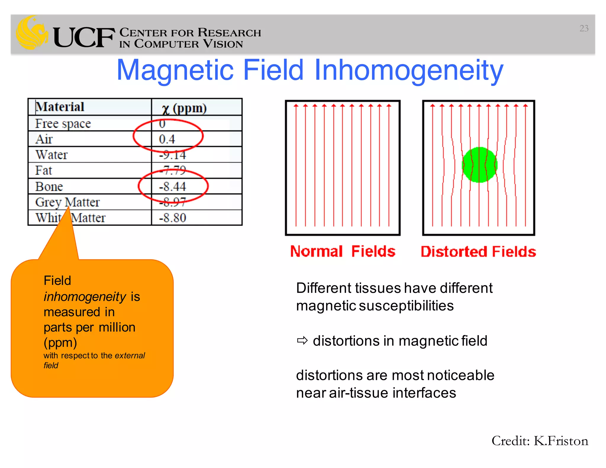
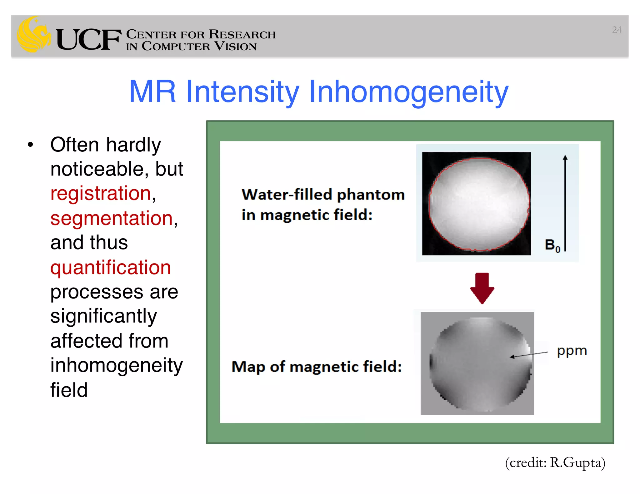
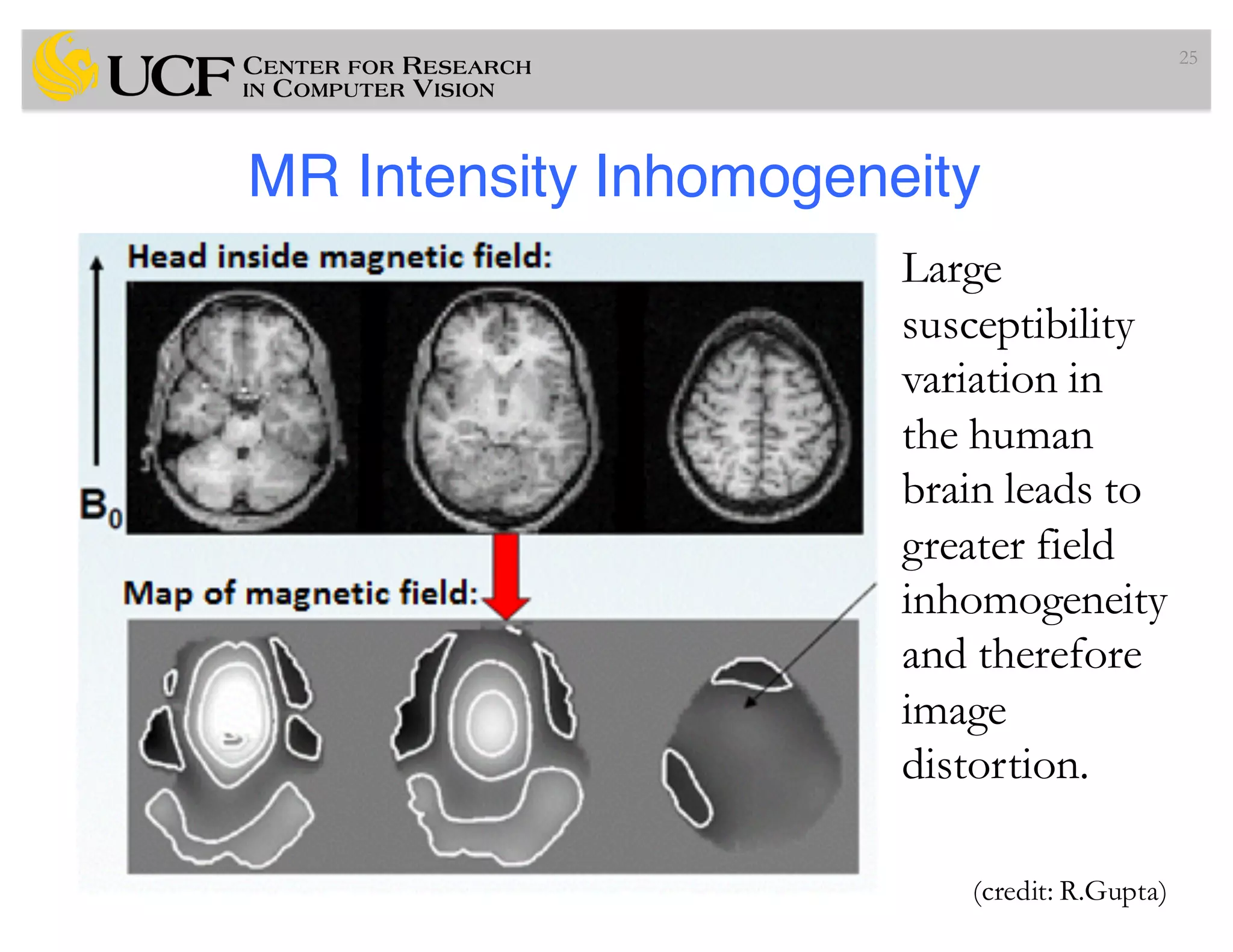
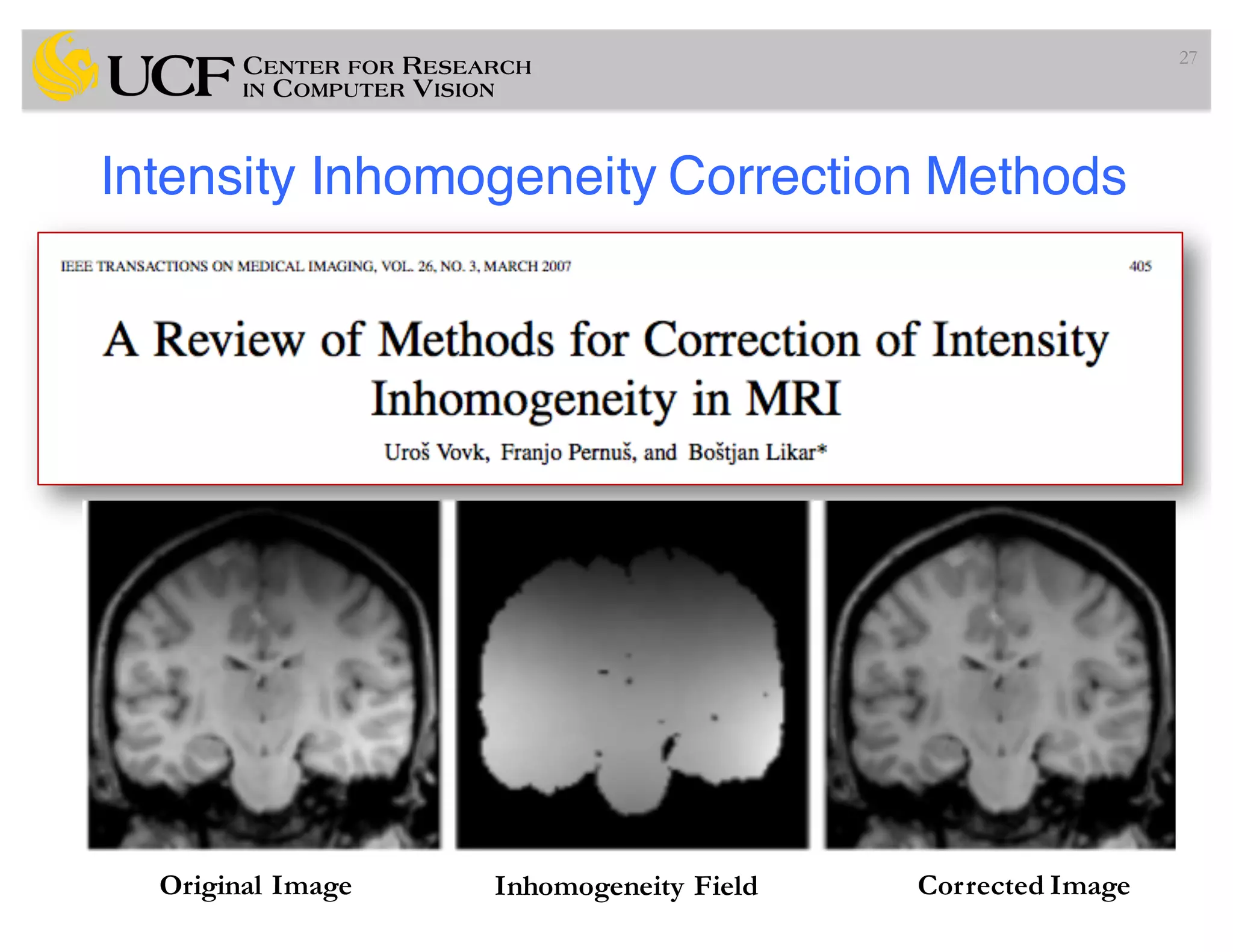
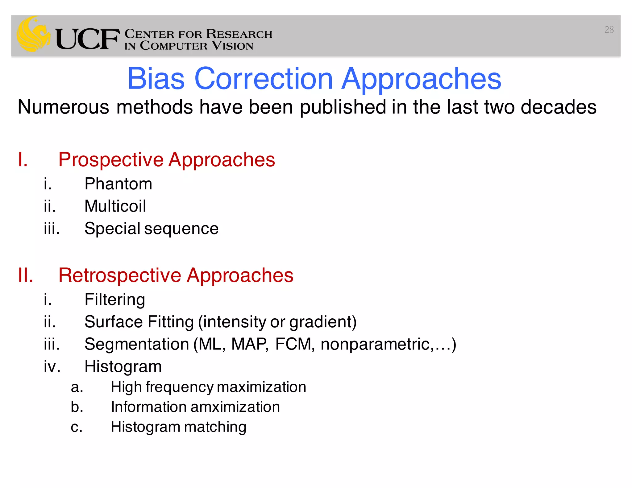
The document outlines the pre-processing techniques in medical image computing, particularly focusing on diffusion-based smoothing and intensity inhomogeneity correction in MRI. It discusses Perona-Malik's anisotropic diffusion method aimed at preserving edges while smoothing images and explores various intensity inhomogeneity correction methods that address challenges in MRI segmentation and analysis. The document also compares prospective and retrospective approaches for correcting these artifacts, emphasizing the need for automated solutions without user intervention.