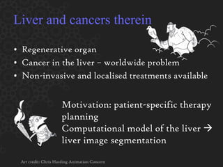
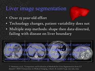
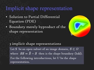
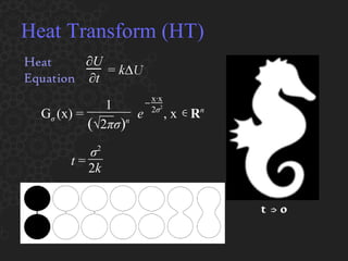
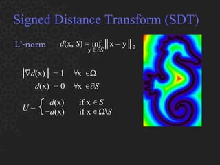
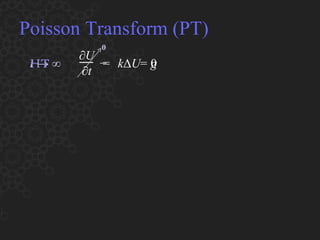
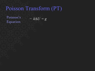
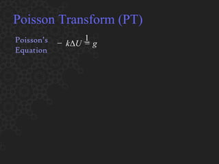
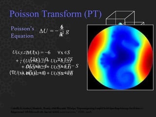
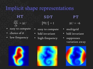
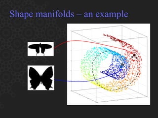
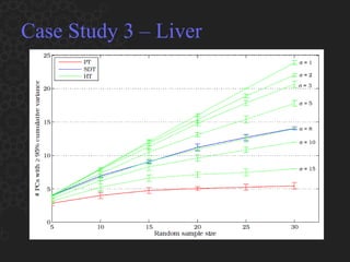
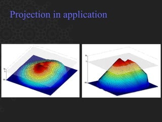
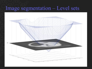
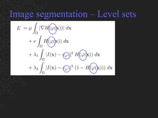
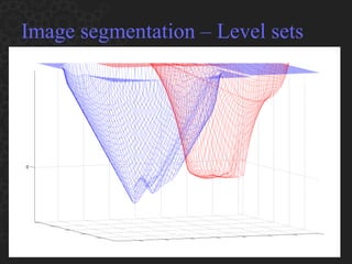
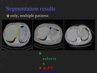
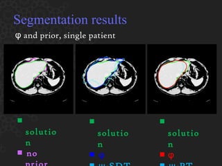
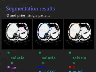
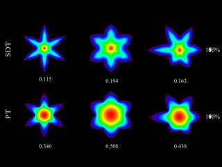
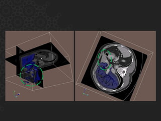
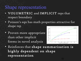
1. The document discusses implicit shape representations for liver segmentation from CT scans, comparing heat, signed distance, and Poisson transforms.
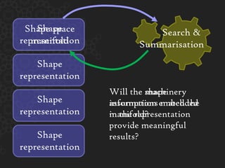
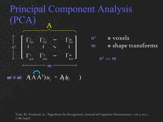
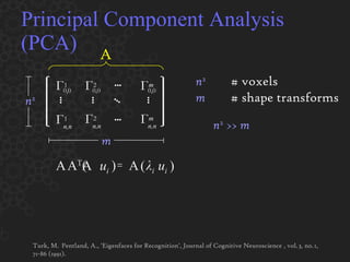
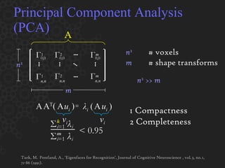
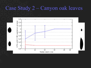
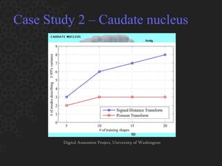
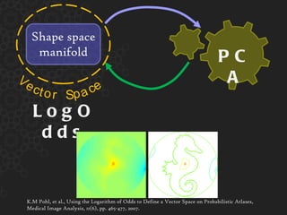
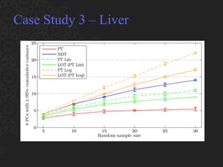
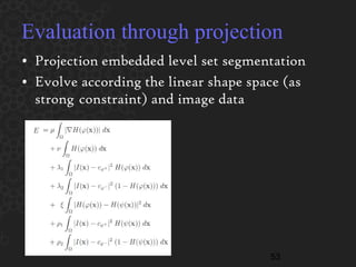
2. It evaluates these representations using principal component analysis to build a linear shape space model from training data.
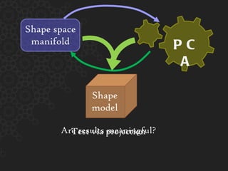
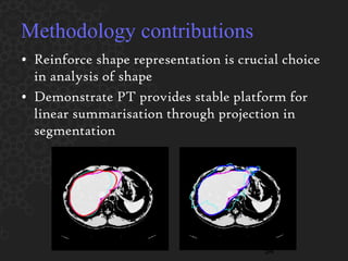
3. Results show the Poisson transform provides the most stable and effective implicit representation for segmentation, outperforming other methods in experiments projecting new shapes into the learned shape space.
13. Poisson Transform (PT) Poisson’s Equation g k 1 Gorelick, Galun, Sharon, Basri, and Brandt, “Shape Representation and Classification Using the Poisson Equation,” PAMI , vol. 28, no. 12, 2006. Cahill, Vesom, Gorelick, Brady, Noble, and Brady, “Investigating Implicit Shape Representations for Alignment of Livers from Serial CT Examinations,” ISBI, 2008. U ( x,y,z ) = 1 6 h 2 − Δ U = 1 6 + ( U ( x + h,y,z ) + U ( x − h,y,z ) + U ( x,y + h,z ) + U ( x,y − h,z ) + U ( x,y,z + h ) + U ( x,y,z − h ) ) Δ U (x) = −6 x S U (x) = 0 Δ U (x) = 6 ⟨ U (x), n (x) ⟩ = 0 x ∂S x T − S x ∂T
14.
15. Will the machinery assumptions match the manifold? Will the shape information embedded in the representation provide meaningful results? Shape representation Search & Summarisation Shape representation Shape representation Shape representation Shape space manifold
17. Principal Component Analysis (PCA) A n 2 # voxels m # shape transforms n 2 >> m Turk, M. Pentland, A., 'Eigenfaces for Recognition', Journal of Cognitive Neuroscience , vol. 3, no. 1, 71-86 (1991). A T A n 2 × n 2 m × m ( ) u i = A ( ) λ i u i n 2 m A Г 0,0 1 ••• ••• Г 0,0 2 Г 0,0 m ••• ••• ••• ••• Г 1 n,n n,n Г 2 n,n Г m
18. Principal Component Analysis (PCA) = A T A A u i A n 2 # voxels m # shape transforms n 2 >> m Turk, M. Pentland, A., 'Eigenfaces for Recognition', Journal of Cognitive Neuroscience , vol. 3, no. 1, 71-86 (1991). ( ) λ i u i ( ) n 2 m A Г 0,0 1 ••• ••• Г 0,0 2 Г 0,0 m ••• ••• ••• ••• Г 1 n,n n,n Г 2 n,n Г m
19. Principal Component Analysis (PCA) = A u i A n 2 # voxels m # shape transforms n 2 >> m Turk, M. Pentland, A., 'Eigenfaces for Recognition', Journal of Cognitive Neuroscience , vol. 3, no. 1, 71-86 (1991). 1 Compactness 2 Completeness ( ) λ i u i v i v i A T A ( ) Σ k i =1 λ i Σ m i =1 λ i < 0.95 n 2 m A Г 0,0 1 ••• ••• Г 0,0 2 Г 0,0 m ••• ••• ••• ••• Г 1 n,n n,n Г 2 n,n Г m
29. PCA LogOdds K.M Pohl, et al., Using the Logarithm of Odds to Define a Vector Space on Probabilistic Atlases, Medical Image Analysis, 11(6), pp. 465-477, 2007. Shape space manifold e t V o r c p c S a e
Prometheus was doomed every day of his eternal life to have his liver eaten by an eagle, which regenerated overnight until he would be saved by Hercules. 1931 Higgins and Anderson pioneered experiment removing 2/3rds of rat liver, where residual lobes grew to compensate for loss in mass in less than a week. Transplanted livers exhibit growth and reduction response according to the organ receiver’s liver cavity. Regenerate through replication of healthy mature liver cells. --------------- Liver and CRC are the 3 rd and 4 th most common causes of cancer-related deaths worldwide as reported in 2002. Liver cancer is relatively uncommon in developed countries, with 82% of cases and deaths occurring in developing countries (due to cofactors of chronic HBV and HCV infections). CRC is the 2 nd most common cause of cancer-related deaths in developed countries. Due to the liver’s blood flow, the liver is a common site of metastatic spread that accounts for 2/3s of CRC deaths. --------------- Many non-invasive and localised treatments are available: radiofrequency ablation, ethanol injection, and embolisation, but they are rarely used without a combination of surgery and chemotherapy. Because they are percutaneous, their efficacy and accuracy is a function of chemical technology, treatment planning, visualisation, and tumour localisation. As the number of treatment options grow and imaging machine technology advances, quantitative and visual knowledge of disease extent is crucial to best provide patient-specific therapy planning. A computational model of the growing number of treatment possibilities and the liver can bridge the gap between the incredible amount of abdominal images per patient.
Liver image segmentation is an old problem with several solutions that continue to change with imaging technology and the advancement of computational power. However, the problem remains difficult because patient variability is always high Patient contrast uptake intensity contrast Patient tumour size/type texture inhomogeneity Patient anatomy shape The most successful liver segmentation methods in recent literature use both prior shape information and boundary-based deformation unassociated with the shape constraint. The secondary step is data-directed, seeking to tailor the first stage result to the specific patient. However, any inhomogeneity exists on the liver border, then the second stage fails to capture the liver, as the shape constraint is no longer applied.
The field of shape representation begin nearly 3 decades ago in the study of visual recognition and perception. What is shape – perceptually, mathematically, computationally? The question of what defines shape changes with respect to the application, can they be related? Can we use information about our cognition to advance computational shape representation? From an object-centred point of view, is shape defined solely by its boundary? Its skeleton? What if there is no clear internal structure? Marr defined 3 criteria for the effectiveness of a shape representation: -- accessibility: how easy is it to capture/compute -- scope/uniqueness (between class): do the shapes in that class have canonical descriptions in the representations? For recognition, we would prefer they be sufficiently unique such that there is no difficulty in distinguishing whether two descriptions specify the same shape -- stability/sensitivity (in-class): similarity between 2 shapes should be reflected in their description but subtle differences must be expressible Additionally Brady added the criteria of rich local support – the idea that it should be information preserving and be capable of being locally computed. What information do we extract from a shape and embed the shape representation? We want the similarity of the shape representation as data to reflect the similarity of the shape itself, as from David Mumford (this is not always obvious) What representation can embed these characteristics of an object’s shape in its representation? For object in question, a shape descriptor should exhibit similarity between suitable shapes, while still articulating acute disparities. In other words, we would like a shape representation that exhibits low and high frequency data about the object’s shape.
There is a very broad spectrum of uses for shape representation. With a growing number of applications and the rise in computing power, computational shape has flourished. They can broadly be divided into explicit and implicit shape representations. Explicit shape representations are representations parameterised as ordered collections of components, such as points, lines, or faces, but can be augmented with additional information. Implicit shape representations assigns a scalar value to every point in space, given a closed, compact shape. The original shape boundary provides a convention or boundary condition for the PDE to be solved. They’re also free of topological constraints and have continuous support throughout the defined space. In an effort to characterise highly variable shape, we introduce 3 well-known or current implicit shape representations. I will show that of the three, the shape representation of the Poisson’s Equation is the best.
The heat eauations is equivalent to the diffusion equation with constant coefficient `k`, where big `U` is the solution and ∆ is the Laplace operator in `n` dimensions. Originally used for scale-space description for zero-crossings of 1-dimensional signals. Then used for scale-based description of planar shapes. An easy way to see how the HT can be used for shape description, parameterised by time, is to imagine that the region in white holds gas particles at constant temperature 100degC and the outer region in black holds gas particles at 0degC at time t = 0. When t > 0, the particles move freely throughout space in Brownian motion, causing temperature diffusion as they gain and lose heat through collisions. How does this give a shape representation? We can glance at the threshold of particles in the region above a given temperature threshold. As time increases, we lose more high-frequency information about the original shape boundary. The HT can be quickly computed by convolving a binary image with the kernel derived from the fundamental solution for the Heat Eq.
A distance is a metric that assigns a scalar value between 2 elements in a set. In Euclidean space, the metric is the L2-norm. It can be approximated by the Eikonal equation with constant cost unity. For shape description, the function provides the minimum Euclidean distance of a point X in space OMEGA to any point on the shape boundary, given the boundary condition. The SDT is easy to compute and is the most widely used implicit shape representation in medical image analysis literature. The concept of using the SDT was borrowed from the level set method, which is a flexible mathematical framework used for image segmentation, One of the key reasons for its popularity is due to its ability to fit into a level-set segmentation framework . In contrast to the HT, the SDT propagates high frequency information of the boundary throughout the representation’s domain. Lipschitz continuity.
Briefly, recall the heat equation. We can add a time-independent energy source `g` and allow the environment to reach an equilibrium of particle diffusion. With time no longer being a variable, the LHS goes to zero and the steady-state temperature of particles at equilibrium is the solution to Poisson’s Equation. In order to solve the PDE, we need to resolve the RHS of Poisson’s Equation. Lena Gorelick first introduced shape representations based on Poisson’s Equation using the analogy of a symmetric Random Walk. For a point x, let U represent the expected number of steps from x to any point on the shape boundary S. In a 3D discrete lattice, that number would be a constant to reach a neighbour plus the average number of steps for x’s neighbours to reach the shape boundary. As it turns out, this is the discrete form of Poisson’s Equation. Then the RHS becomes -6, with step size h = 1. If a particle were outside the shape, then it might not ever reach the boundary in a random walk. Then the analogy fails, and Poisson’s equations has infinitely many solutions. In order to extend the shape representation to the shape exterior, we define an open sphere T in the image space Omega, centred on the shape. We prescribe Neumann boundary condition on the boundary of the sphere `T`. In the random walk analogy, the particle would reflect in the direction normal to the sphere in a symmetric random walk. Computing the PT on arbitrary boundaries in 3D requires the use of a Multi-grid algorithm. the dot product with the normal is the flow through the boundary,
In summary, The HT is easy to compute But has high-curvature erosion, leaving low-frequency data in the representation, and the shape’s resultant topology is parameterised by the choice of sigma. The SDT is also easy to compute and boundary invariant, But has variation propagation beyond the neighbourhood of occurrence, projecting high frequency data throughout the image space The PT is not as easy to compute, requiring a multigrid method in 3D (although once can do a direction solution in 2D). It is however boundary invariant, and regularises boundary variations increasingly as you move away from the boundary. We can see the effects of each equation on the shape representation given the orignaly boundary by looking at the contour plots, where every contour represents a tenth interval of the representation’s range.
If we were looking at several species of seahorse shapes, the would comprise a class of shapes. If we use a specific shape representation to describe the class, they form a shape manifold in shape space. If each shape representation is parameterised by 20 points, then the shape space is 20-dimensional, however the manifold they embed usually has a smaller, intrinsic dimension. When we encounter a new shape, does it belong? If so, where in the space does it belong? What is it most similar to? Can we do this without comparing to all the shapes in our sample subset? We use automatic methods to search and summarise the shape manifold. These seek to find the intrinsic dimension of the shape manifold. There are numerous methods, as each one makes certain assumptions about the data. The information about shape that is embedded in the representations, changes the structure of the manifold. We want a canonical description, in an implicit shape model – so we do summarisation. But what method do we use? It depends on what the underlying data looks like – very hard to do!
A class of shapes (say a class of pear shapes or a class of banana shapes) is said to exist on a manifold `M`, where every point in `M` represents a shape. We would like to know how to best characterise a manifold spanned by implicit shapes. The dimension of `M` is determined by the dimension of the shape representation it has embedded. For example, if the shape is comprised of 20 points, then `M` is 20-dimensional. In application, these maniforlds are thought to have an intrinsic dimension `k` such that k << d. The process by which `k` is sought is called manifold learning or dimensionality reduction. The swiss roll is a popular example – while existing in 3D, the intrinsic dimension is only 2. In an simple example, suppose we have to very different shapes from a single class – Lepidoptera. Using a simple L2-metric, the distance between them in 3D might not accurately reflect how different these shapes are...which is more accurately measured in the distance of the intrinsic 2D space. These methods are not only applied to shape spaces, but to manifolds in image spaces and space with high-dimensional vectorised data. There are numerous linear and non-linear methods to do dimensionality reduction. While any of these methods can arguably be more suitable for shape anaylsis, we wish to show that a shape representation that suppresses redundancy in variability yet elicits distinguishing global features will result in more meaningful results.
The machinery we chose to summarise our data is PCA. It’s widely used, easy to compute and interpret. The intrinsic dimension of a shape space is found by calculating the dominant eigenvectors (called principal components) from a covariance matrix of the sample shapes. We select the intrinsic dimension `k` such that `k` principal components summaries at least 95% of the variance from the sample shapes. These principal components seek to maximise the variance across the given data set by minimising the mean square error between the data and the PCs. Minimise the MSE by finding the eigenvalues and eigenvectors of the covariance. Assumes the data points have a Gaussian distribution. What does `k` tell us about the data??
Shape space manifolds may not be closed vector spaces, but they form connected manifolds (because perturbing the boundary by e, changes the sahpe rep by small amount). By definition, the SDT will propagate bdd variations throughout the domain, which can make 2 shapes by SDT representation appear less similar than the original shapes they represent. In each individual shape representation, boundary variations are generated throughout the domain, beyond the neighbourhood of the boundary and necessity. Redundancies across the class population give rise to class similarities, which are desirable when characterising a class of shapes. In the case of the PT, the interior regularisation property provides redundancies across the class, giving rise to a canonical description. Because the SDT lacks the regularisation property away from the boundary, the largest variations near the boundary are eclipsed in PCA by variations existing throughout the entire domain. Uniqueness: poisson eqn is a scalar function that on a bdd domain is uniquely defined by its value on the bdd and its laplacian in the interior (perez msft res UK 2003) **variation propagation beyond neighborhood of occurrence
If we were looking at several species of seahorse shapes, the would comprise a class of shapes. If we use a specific shape representation to describe the class, they form a shape manifold in shape space. If each shape representation is parameterised by 20 points, then the shape space is 20-dimensional, however the manifold they embed usually has a smaller, intrinsic dimension. When we encounter a new shape, does it belong? If so, where in the space does it belong? What is it most similar to? Can we do this without comparing to all the shapes in our sample subset? We use automatic methods to search and summarise the shape manifold. These seek to find the intrinsic dimension of the shape manifold. There are numerous methods, as each one makes certain assumptions about the data. The information about shape that is embedded in the representations, changes the structure of the manifold. We want a canonical description, in an implicit shape model – so we do summarisation. But what method do we use? It depends on what the underlying data looks like – very hard to do!
By projection, we mean infer a new shape from the newly resolved lower-dimensional shape space.
Image segmentation seeks to partition an image for further analysis. The wide variety of applications precludes a general solution. The level set method uses a higher-dimensional interface to partition a region. And driven by speed functions.
12% improvement on Dice measure, 40% improvement on Hausdorff measure Dice: S = 2(X intersect Y) / (X + Y) Hausdorff meausre: Max(sup inf d(x,y), sup inf d(x,y)) For each x in X, find the min dist to Y, then give the sup of x in X
For anatomical object segmentation using level-sets (LS), shape priors are often employed. Shape spaces are created using the SDT for ease of integration into LS frameworks and summarized with Principal Components Analysis.
My contibutions include -Proving that shape representation is a crucial choice in shape analysis. -I also showed that a shape class represented with the Poisson Transform can be linearly approximated with PCA for summarisation. Additionally, we can infer new shapes in linear projection for segmentation.