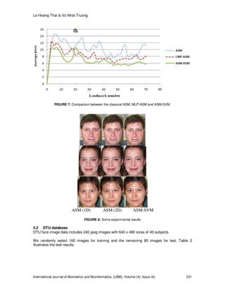
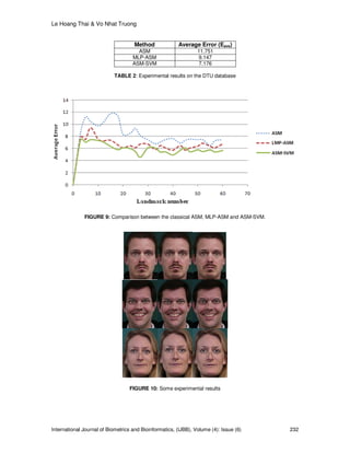
The document proposes improvements to the classical Active Shape Model (ASM) algorithm for face alignment. The improvements include: 1) Combining Sobel filtering and 2D profiles to build texture models, 2) Applying Canny edge detection for enhancement, 3) Using Support Vector Machines (SVM) to classify landmarks for more accurate localization, and 4) Automatically adjusting 2D profile lengths based on image size. Experimental results on two face databases show the proposed ASM-SVM method achieves better alignment accuracy than the classical ASM and other methods.
![Le Hoang Thai & Vo Nhat Truong
International Journal of Biometrics and Bioinformatics, (IJBB), Volume (4): Issue (6) 224
Face Alignment Using Active Shape Model And Support Vector
Machine
Le Hoang Thai lhthai@fit.hcmus.edu.vn
Department of Computer Science
University of Science
Hochiminh City, 70000, VIETNAM
Vo Nhat Truong vntruong@gmail.com
Faculty/Department/Division
University of Science
Hochiminh City, 70000, VIETNAM
Abstract
The Active Shape Model (ASM) is one of the most popular local texture models
for face alignment. It applies in many fields such as locating facial features in the
image, face synthesis, etc. However, the experimental results show that the
accuracy of the classical ASM for some applications is not high. This paper
suggests some improvements on the classical ASM to increase the performance
of the model in the application: face alignment. Four of our major improvements
include: i) building a model combining Sobel filter and the 2-D profile in searching
face in image; ii) applying Canny algorithm for the enhancement edge on image;
iii) Support Vector Machine (SVM) is used to classify landmarks on face, in order
to determine exactly location of these landmarks support for ASM; iv)
automatically adjust 2-D profile in the multi-level model based on the size of the
input image. The experimental results on Caltech face database and Technical
University of Denmark database (imm_face) show that our proposed
improvement leads to far better performance.
Keywords: Face Alignment, Active Shape Model, Principal Component Analysis.
1. INTRODUCTION
Face recognition is the problem to search human faces in large image database. In detail, a face
recognition system with the input of an arbitrary image will search in database to output people’s
identification in the input image. The face recognition system’s stages are illustrated in Figure 1
[5].
FIGURE 1: Structure of a face recognition system.](https://image.slidesharecdn.com/ijbb-81-160207144220/85/Face-Alignment-Using-Active-Shape-Model-And-Support-Vector-Machine-1-320.jpg)
![Le Hoang Thai & Vo Nhat Truong
International Journal of Biometrics and Bioinformatics, (IJBB), Volume (4): Issue (6) 224
Face Alignment Using Active Shape Model And Support Vector
Machine
Le Hoang Thai lhthai@fit.hcmus.edu.vn
Department of Computer Science
University of Science
Hochiminh City, 70000, VIETNAM
Vo Nhat Truong vntruong@gmail.com
Faculty/Department/Division
University of Science
Hochiminh City, 70000, VIETNAM
Abstract
The Active Shape Model (ASM) is one of the most popular local texture models
for face alignment. It applies in many fields such as locating facial features in the
image, face synthesis, etc. However, the experimental results show that the
accuracy of the classical ASM for some applications is not high. This paper
suggests some improvements on the classical ASM to increase the performance
of the model in the application: face alignment. Four of our major improvements
include: i) building a model combining Sobel filter and the 2-D profile in searching
face in image; ii) applying Canny algorithm for the enhancement edge on image;
iii) Support Vector Machine (SVM) is used to classify landmarks on face, in order
to determine exactly location of these landmarks support for ASM; iv)
automatically adjust 2-D profile in the multi-level model based on the size of the
input image. The experimental results on Caltech face database and Technical
University of Denmark database (imm_face) show that our proposed
improvement leads to far better performance.
Keywords: Face Alignment, Active Shape Model, Principal Component Analysis.
1. INTRODUCTION
Face recognition is the problem to search human faces in large image database. In detail, a face
recognition system with the input of an arbitrary image will search in database to output people’s
identification in the input image. The face recognition system’s stages are illustrated in Figure 1
[5].
FIGURE 1: Structure of a face recognition system.](https://image.slidesharecdn.com/ijbb-81-160207144220/75/Face-Alignment-Using-Active-Shape-Model-And-Support-Vector-Machine-1-2048.jpg)
![Le Hoang Thai & Vo Nhat Truong
International Journal of Biometrics and Bioinformatics, (IJBB), Volume (4): Issue (6) 225
The face alignment is one of important stages of the face recognition. Moreover, face alignment is
also applied for other face processing applications; such as face modeling and synthesis. Its
objective is to localize the feature points on face images such as the contour points of eye, nose,
mouth and face (illustrated in Figure 2).
FIGURE 2: Face alignment.
There are many face alignment methods. Two popular face alignment methods are Active Shape
Model (ASM) [16] and Active Appearance Model (AAM)[8] are proposed by Cootes et al.
The two methods use a statistical model to parameterize a face shape with Principal Component
Analysis (PCA) method. However, their feature model and optimization are different. ASM
algorithm has a 2-stage loop: in the first stage, given the initial labels, searching for a new
position for every label point in its local region which best fits the corresponding local 1-D profile
texture model; in the second stage, updating the shape parameters which best fits these new
label positions. AAM method uses its global appearance model to directly conduct the
optimization of shape parameters. Owing to the different optimization criteria, ASM performs
more precisely on shape localization, and is quite more robust to illumination and bad
initialization. In the paper extent, we develop the classical ASM method to create a new method
named ASM-SVM which has achieved better results.
Because ASM only uses a 1-D profile texture feature, which is not enough to distinguish feature
points from their local regions, the ASM algorithm often fall into local minima problem in the local
searching stage. A few representative texture features and pattern recognition methods are
proposed to reinforce the ASM local searching, e.g. Gabor wavelet, Haar wavelet, Ranking-
Boost, Fisher Boost and MLP-ASM (Perceptron network) [5]. Nevertheless, an accurate local
texture model to large data sets is still unachieved target.
In this paper, we propose the improvements in the local search of ASM. The main improvements
are followed: first, build a model combining Sobel filter and the 2-D profile in searching face in
image; second, applying Canny algorithms for the enhancement edge in image; third, support
vector machine (SVM) is used to classify landmarks on face, in order to determine the exact
location of these landmarks support for ASM; last, automatically adjust 2-D profile in the multi-
level model based on the size of the input image.
The paper is structured as follows: Section 2, we present the classical ASM algorithm, section 3
presents details of our improvements and Section 4 presents experimental results and Section 5
presents conclusion and future works.
2. CLASSICAL ASM ALGORITHM
2.1 Training stage
A shape can be represented by n points {(xi, yi)} as a 2n-D element vector, X = (x1, y1, …, xn, yn)
T
.
With training shape S (S = {Xi}), we perform statistical shape on the same coordinates.](https://image.slidesharecdn.com/ijbb-81-160207144220/85/Face-Alignment-Using-Active-Shape-Model-And-Support-Vector-Machine-2-320.jpg)
![Le Hoang Thai & Vo Nhat Truong
International Journal of Biometrics and Bioinformatics, (IJBB), Volume (4): Issue (6) 226
FIGURE 3: Local features to be built in the period of training (a) typical 1-D (b) typical 2-D
The shape of the training set S are aligned by algorithms Generalized Procrustes Analysis (GPA)
[12]. Average shape ( x ) is the average shape vector of all alignment shape. PCA is applied to
calculate this shape and the covariance matrix is chosen so that accounted for 97.5% of the total
value of training set that are arranged from large to small and used to store as the corresponding
eigenvector matrix (P).
In next stage, we determine the gray level to create the statistical model of gray level around the
landmarks to build a subspace represents the change of training shape. 1-D profiles are
constructed by the gray level of points on the line with fixed length. These straight lines are
orthogonal to the edge of this shape at the landmark. The gray level sample is stored as a vector
that is then standardized by replacing each element of the vector with the intensity of gray levels
(the difference of gray level at that point and the preceding point) and then dividing the magnitude
of the vector average. Average profile (of all files in training set) is called average profile vector
( g ) and covariance matrix of all the vector present as Sg. Average profile vector and covariance
matrix are generated for each point and three level of the pyramid model (each image in the
pyramid is half the image size of it before).
Similar, training data can be calculated by 2-D profile that is created at each landmark by the
derivation of gray level image (the sum of square derivation in x and y directions) .Result matrix is
transformed into a vector and then normalized by the sigmoid transformation for each specific
element of profile g'i as follow equation:
)(
'
qg
g
g
i
i
i
+
= (1)
q: const.](https://image.slidesharecdn.com/ijbb-81-160207144220/85/Face-Alignment-Using-Active-Shape-Model-And-Support-Vector-Machine-3-320.jpg)
![Le Hoang Thai & Vo Nhat Truong
International Journal of Biometrics and Bioinformatics, (IJBB), Volume (4): Issue (6) 227
FIGURE 4: Illustrate local features: (a) typical 1D and (b) typical 2D
Using 1-D profile to find landmark in some cases is not accurate. For example, Figure 4(a)
illustrates the case that desired position is P1. However, 1-D profile achieves P2 point instead of
P1. Hence, 2-D profile is necessary to solve this problem (Figure 3 (b)). The desired location is
P1 can be determined exactly by 2-D profile. Moreover, misplaced errors will reduce by using 2-D
profile.
2.2 Alignment stage
In alignment phase, faces in test images will be identified in first step. Face detection algorithm,
Viola Jones in OpenCV [11], is used for this step. After detecting the location of faces in images,
similar transformations (scale, rotation and translation) will operate on the shape model that
represent the face (constructing from the training data set) to fit this model to test face (the face is
detected by OpenCV). Achieving shape will use as initial shape. A loop on the initial shape would
be made to find suitable final landmark. These landmarks will form a shape that best suits the
considered face image.
Typical multi-level model is built for image at each level by the method as in training phase. The
process of identifying profile start from the lowest level of the pyramid (level 2) and gradually
move up to the highest level (level 0) (Figure 4). Fluctuations of the landmarks are highest at the
lowest level and they are smaller at higher levels. Best location of the landmark is determined by
establishing the profile of the candidate neighboring around the landmarks. The candidate points
that have nearly all features of average landmark will be selected as the new location of
landmark. The weighting function that use in ASM to determine at this landmark is the smallest
Mahalanobis distance (f1(g)) of candidates (g) with average profile g by the following equation:
)()()( 1
1 ggSggxf g
T
−−= −
(2)
Searching process on the 2-D profile with size 15x15 pixels around the landmark will operate at
all levels of multi-level model.
When all landmarks move to the best location, a new shape (xi) needs to be converted into an
appropriate shape and to represent the boundary of face. This is done by Equation (3).
PbxxL += (3)
xL: the closest shape vector (xI)
x : average shape
P: eigenvector matrix](https://image.slidesharecdn.com/ijbb-81-160207144220/85/Face-Alignment-Using-Active-Shape-Model-And-Support-Vector-Machine-4-320.jpg)
![Le Hoang Thai & Vo Nhat Truong
International Journal of Biometrics and Bioinformatics, (IJBB), Volume (4): Issue (6) 228
b: coefficient vector that is predicted to generate the face shape.
b is calculated by performing a loop so that the distance of formula (4) is the smallest.
))(,( PbxTxdist I + (4)
T is a transformation that makes minimizing distance between xI and Pbx + . [9] represents the
algorithm that finds b and T. When we get vector b, bi is ith
element of vector b and it have to be
between iλα− and iλα+ with α is 3 and iλ is ith
eigenvalue.
The limitation of these values can ensure that the generated shape is similar to those in the
original training set.
At each level of multi-level model, a loop will be done until convergence (no significant change of
landmark position in two consecutive loops). If convergence is done at lowest level,the shape will
be changed by scale transformation and used as initial position for the next level of multi-level
model. This process continues until convergence and achieving final landmarks at the highest
level of multi-level model.
FIGURE 5: Illustrate alignment of multi-level model](https://image.slidesharecdn.com/ijbb-81-160207144220/85/Face-Alignment-Using-Active-Shape-Model-And-Support-Vector-Machine-5-320.jpg)
![Le Hoang Thai & Vo Nhat Truong
International Journal of Biometrics and Bioinformatics, (IJBB), Volume (4): Issue (6) 229
3. IMPROVEMENT FOR ASM
3.1 Combining 2-D profile and Sobel filter
In order to balance brightness in image as well as distinguish between high and low frequency
variations in image. In this paper, we determine the 2-D profile for each point by combining
histogram equalization and Sobel filter as follow:
Step 1: Using the Histogram balancing algorithm to normalize brightness of image.
Step 2: Using the Sobel filter function in two directions x, y. Constructing texture matrix, with
value of each point in the matrix is the square root of the sum of squared derivative in two
directions (x and y).
Step 3: Normalizing result matrix to a vector by formula (5).
∑
=
i
i
i
g
g
g' (5)
3.2 Enhancement edge by Canny algorithm
To increase more accurately for fitting points that lie along the boundary, we use the weighting
function (6).
)())(()( 1
2 ggSggcgf g
T
−−Ι−= −
(6)
In the function f2(g), Ι is the gray value at candidate point and has value 0 (for the point not on
the boundary) or 1 (for the point on the boundary). Ι determined based on enhancement edge by
Canny algorithm [11]. c is a constant and we choose 2 for our experiments. Function f2(g) can
increase the ability to searching landmark on the boundary of shape that hard to find in classical
algorithm.
FIGURE 6: Illustrates the edge detection algorithm (Canny): (a) original image (b) resulting image
3.3 Applying SVM to find landmarks
In the classical ASM method, the PCA does not consider the distinction between the positive
sample (the points represent the model (Section 4)) and negative sample (the points are not
positive sample). So the searching landmark process often falls into local extreme values. To
distinguish between positive sample and negative sample, we chose SVM method [10] because
this method generalizes learning sample (without learning much data as other classification
methods) and minimizes the structure error that increases the classified ability. In this paper, we
use linear SVM.
For each point, we determine local 2-D profile with this. Next, the positive samples (the landmark)
are selected from the focal point, whereas the negative samples (the point is not the landmark)
randomly select window which has same size and different focal point with positive sample.
Algorithms search candidate around the current landmark to determine the new landmark:](https://image.slidesharecdn.com/ijbb-81-160207144220/85/Face-Alignment-Using-Active-Shape-Model-And-Support-Vector-Machine-6-320.jpg)